Diagnostic Checking, Time Series and Regression

(1)

Western University Western University

Scholarship@Western

Electronic Thesis and Dissertation Repository

7-28-2011 12:00 AM

Diagnostic Checking, Time Series and Regression

Esam Mahdi

The University of Western Ontario Supervisor

A.I. McLeod

The University of Western Ontario

Graduate Program in Statistics and Actuarial Sciences

A thesis submitted in partial fulfillment of the requirements for the degree in Doctor of Philosophy

Follow this and additional works at: https://ir.lib.uwo.ca/etd

Part of the Applied Statistics Commons, Longitudinal Data Analysis and Time Series Commons, and the Multivariate Analysis Commons

Recommended Citation Recommended Citation

Mahdi, Esam, "Diagnostic Checking, Time Series and Regression" (2011). Electronic Thesis and Dissertation Repository. 244.

https://ir.lib.uwo.ca/etd/244

This Dissertation/Thesis is brought to you for free and open access by Scholarship@Western. It has been accepted for inclusion in Electronic Thesis and Dissertation Repository by an authorized administrator of

(2)

DIAGNOSTIC CHECKING, TIME SERIES AND REGRESSION

(Spine title: Diagnostic Checking, Time Series and Regression)

(Thesis format: Integrated-Article)

by

Esam Mahdi

Graduate Program in

Statistics

A thesis submitted in partial fulfillment of the requirements for the degree of

Doctor of Philosophy

The School of Graduate and Postdoctoral Studies The University of Western Ontario

London, Ontario, Canada

(3)

(4)

ABSTRACT

In this thesis, a new univariate-multivariate portmanteau test is derived. The

proposed test statistic can be used for diagnostic checking ARMA , VAR , FGN ,

GARCH , and TAR time series models as well as for checking randomness of series

and goodness-of-fit VAR models with stable Paretian errors. The asymptotic

distri-bution of the test statistic is derived as well as a chi-square approximation. However,

the Monte-Carlo test is recommended unless the series is very long. Extensive

sim-ulation experiments demonstrate the usefulness of this test and its improved power

performance compared to widely used previous multivariate portmanteau diagnostic

check.

The contributed R package portes is also introduced. This package can utilize

multi-core CPUs often found in modern personal computers as well as a computer

cluster or grid. The proposed package includes the most important univariate and

multivariate diagnostic portmanteau tests with the new test statistic given in this

thesis. It is also useful for simulating univariate/multivariate data from nonseasonal

ARIMA /VARIMA process with finite or infinite variances, testing for stationarity and

invertibility, and estimating parameters from stable distributions. Many illustrative

applications are given.

In this thesis, it has been shown that the classical ordinary least squares regression

may produce smaller p-values than it should due to the lack of statistical independency

in the fitted model which may invalidate the statistical inferences. The Poincar´e plots

are suggested to check for such hidden positive correlations.

KEY WORDS: Diagnostic check, Portmanteau test, Monte-Carlo significance test,

Residual autocorrelation function, VARMA models, FGN models, GARCH models,

(5)

ACKNOWLEDGEMENTS

I reserve my greatest appreciation for my thesis supervisor, Professor A.I. McLeod,

for suggesting the research topics, his extremely helpful guidance, encouragement and

patience throughout the course of my research work. I would like also to thank my

thesis examiners, Professors Rogemar Mamon, Serge B. Provest, John Knight, and

Yulia Gel for all helpful comments and suggestions. Finally, I would like to thank my

(6)

LIST OF TABLES

1.1 The empirical 1% and 5% significance levels, in percent, comparing approximation, aχ2_b, and Monte-Carlo, MC, for the portmanteau test

statisticDm. . . 20

1.2 Empirical power in percent comparison ofDm and ˜Qm for nominal 1% and 5% tests. 104 simulations with N = 103. . . 25

1.3 IBM and S&P 500 Index Data. aχ2_b: approximation. MC: Monte-CarloN = 103. NA: not applicable. The p-values are in percent. The ∗ indicates a p-value less than 0.1%. . . 27

1.4 Trivariate West German Macroeconomic Series. aχ2_b: approximation. MC: Monte-Carlo using 103 replications. The p-values are in percent and ∗ indicates a p-value less than 0.1%. . . 27

1.5 The residuals of the fitted VAR(2) model on West German Macroeco-nomic series are tested for heteroscedastic effects. aχ2_b: approximation. MC: Monte-Carlo using 103 replications. The p-values are in percent and ∗ indicates a p-value less than 0.1%. . . 28

2.1 CPU time in seconds. The R functions FitAR(), ar(), arima(), arima0(), Arima(), and auto.arima() are used to fit the AR (1) model to univariate time series of lengths n = 100,500,1000 and the portest() function is applied on the fitted model based on 103 repli-cations of Monte-Carlo test. nslaves denotes the number of CPU’s are used. . . 43

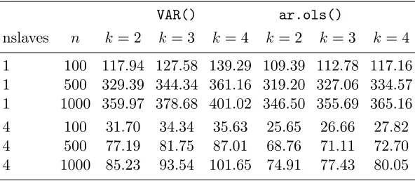
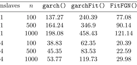
2.2 CPU time in seconds. TheR functions VAR() and ar.ols()are used to fit the VAR (1) model to series of lengths n = 100,500,1000 with dimensionsk= 2,3,4.Theportest()function is applied on the fitted model based on 103 replications of Monte-Carlo test. nslaves denotes the number of CPU’s are used. . . 43

2.3 CPU time in seconds. Univariate time series of lengthsn= 100,500,1000 are generated from normal process andRfunctionsgarch()and garch-Fit() are used to fit the GARCH (1,1) model, whereas the function FitFGN() is used to fit FGN model. The portest() function is ap-plied on the fitted model based on 103 replications of Monte-Carlo test. nslaves denotes the number of CPU’s are used. . . 44

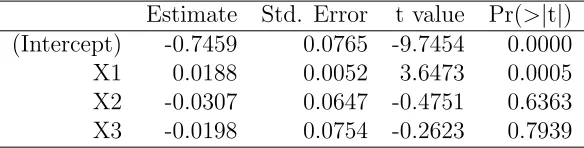
3.1 Classical ordinary least squares model (OLS). . . 81

3.2 Generalized least squares model (GLS) with exact covariance. . . 82

(9)

3.4 Distance vector generated fromU(0,1); k=1, range = 3, 6, 9, and n=60. . 94

3.5 Distance vector generated fromN(0,1); k=1, range = 3, 6, 9, and n = 90. 95

3.6 Distance vector generated fromN(0,1); k=2, range = 3, 6, 9, and n=30. 96

(10)

LIST OF FIGURES

2.1 A simulated time series of example 2.5.2.2. . . 71

2.2 A simulated time series of example 2.5.2.3. . . 72

3.1 Poincar´e plot of the residuals from OLS fitted model with a loess smooth. 82

3.2 Poincar´e plot of the residuals from GLS fitted model with a loess smooth. 83

3.3 Poincar´e plot of deviance residuals in the logistic regression of low birth weight on 9 explanatory variables and 8 parametric bootstrap simulations. 85

3.4 Residual dependency plot of residuals vs. age. . . 86

3.5 Residuals plot in the robust loess fit of Cleveland (1993, section 3.6) to the polarization data.. . . 87

3.6 Poincar´e plot of residuals in the robust loess fit to the polarization data. . 87

(11)

INTRODUCTION

After identification and estimation of the parameters in a fitted model, the

good-ness of fit test is the next most important step for testing the selected model. In time

series analysis, we assume that the series is stationary with white noise innovations.

This implies that a good fitted model must produce residuals that are approximately

uncorrelated in time. Box and Pierce(1970) show that the asymptotic distribution of

the residual autocorrelations can be utilized to check the validity of this assumption

under the ARMA models. They introduced to the literature the overall

goodness-of-fit test on the residuals autocorrelations up to lag m. This test statistic is called

portmanteau test. Since then there evolves many literature on portmanteau tests

for ARMA and GARCH models (Ljung and Box, 1978; McLeod and Li, 1983; Peˇna

and Rodriguez, 2002; Rodr´ıguez and Ruiz, 2005; Peˇna and Rodriguez, 2006). The

portmanteau test is extended to the multivariate VARMA models by Chitturi (1974,

1976); Hosking (1980); Li and McLeod (1981); Francq and Ra¨ısi (2007) and to the

MGARCH models by (Li and Mak,1994;Ling and Li,1997). Lin and McLeod(2006)

introduce the Monte-Carlo portmanteau test and show that this test provides a test

with the correct size. They show that the Monte-Carlo version ofPeˇna and Rodriguez

(2002) is often more powerful than its competitors. Lin and McLeod(2008) extends

the Monte-Carlo test ofPeˇna and Rodriguez(2002) to the ARMA models with stable

Paretian errors.

In Chapter 1 of this thesis we introduce a new univariate-multivariate

portman-teau test based on the approximation chi-square distribution and the Monte-Carlo

procedures. The new test statistic may be considered an extension of the univariate

(12)

(2006,2008). Simulation experiments demonstrate that the proposed test statistic is

the most powerful test with the correct size.

In Chapter 2, the portmanteau tests for time series models, portes, R package

is introduced. The Simple Network of Workstations, snow, R package for parallel

computing is implemented in this package. Many applications with this package are

given.

In Chapter 3, the Poincar´e plots are suggested as a tool for checking the

possi-bility of lack of statistical independence in the observations due to positive hidden

correlations. It is found via simulations that the test statistics based on the classical

ordinary least squares regression may overstate the significance level due to lack of

(13)

REFERENCES

Box, G. and Pierce, D. (1970). Distribution of residual autocorrelation in autoregressive-integrated moving average time series models. Journal of Ameri-can Statistical Association 65(332), 1509–1526.

Chitturi, R. V. (1974). Distribution of residual autocorrelations in multiple autore-gressive schemes.Journal of the American Statistical Association 69(348), 928–934.

Chitturi, R. V. (1976). Distribution of multivariate white noise autocorrelations.

Journal of the American Statistical Association 71(353), 223–226.

Francq, C. and Ra¨ısi, H. (2007). Multivariate portmanteau test for autoregressive models with uncorrelated but nonindependent errors.Journal of Time Series Anal-ysis 28(3), 454–470.

Hosking, J. R. M. (1980). The multivariate portmanteau statistic. Journal of Amer-ican Statistical Association 75(371), 602–607.

Li, W. K. and Mak, T. K. (1994). On the squared residual autocorrelations in non linear time series with conditional heteroskedasticity. The Journal of Time Series Analysis 15, 627–636.

Li, W. K. and McLeod, A. I. (1981). Distribution of the residual autocorrelation in multivariate arma time series models. Journal of the Royal Statistical Society, Series B 43(2), 231–239.

Lin, J.-W. and McLeod, A. I. (2006). Improved Peˇna-Rodr´ıguez portmanteau test.

Computational Statistics and Data Analysis 51(3), 1731–1738.

Lin, J.-W. and McLeod, A. I. (2008). Portmanteau tests for ARMA models with infinite variance. Journal of Time Series Analysis 29(3), 600–617.

Ling, S. and Li, W. K. (1997). Diagnostic checking of nonlinear multivariate time series with multivariate ARCH errors. Journal of Time Series Analysis 18(5), 447–464.

Ljung, G. M. and Box, G. E. P. (1978). On a measure of lack of fit in time series models. Biometrika 65, 297–303.

(14)

Peˇna, D. and Rodr´ıguez, J. (2002). A powerful portmanteau test of lack of test for time series. Journal of American Statistical Association 97(458), 601–610.

Peˇna, D. and Rodr´ıguez, J. (2006). The log of the determinant of the autocorrelation matrix for testing goodness of fit in time series. Journal of Statistical Planning and Inference 8(136), 2706–2718.

(15)

IMPROVED MULTIVARIATE PORTMANTEAU TEST

Chapter 1 IMPROVED MULTIVARIATE PORTMANTEAU TEST

1.1 INTRODUCTION

The VARMA (p, q) model for ak-dimensional mean zero time seriesZt = (Z1,t, . . . , Zk,t)0

can be written as

Φ(B)Zt =Θ(B)at, (1.1)

where Φ(B) = _I_k−Φ₁B− · · · −ΦpBp,Θ(B) = Ik −Θ1B− · · · −ΘqBq, Ik is

the identity matrix of order k, the coefficient matrices are, Φ_` = (φ_i,j,`)_k_×_k, ` =

1, . . . , p; Θ_` = (θ_i,j,`)_k_×_k, ` = 1, . . . , q and B is the backshift operator on t. Let

β= (vecΦ1, . . . ,vecΦp,vecΘ1, . . . ,vecΘq) be the vector of true parameters, where

vec denotes the matrix vectorization function. We assume that an efficient estimation

algorithm such as maximum likelihood is used to produce the corresponding estimate

ˆ

β so that ˆβ −β = Op(n−1/2). The white noise process, at = (a1,t, . . . , ak,t)0, is

assumed independent normal with mean zero and covariance matrix, E(ata0_t₋_`) =

δ_`Γ0, whereΓ0 is the innovation covariance matrix andδ` = 1 or 0 according as` = 0

or `6= 0. The assumption of normality may be relaxed to that of strong white noise

so that at, t = 1, . . . , n are assumed to be independent and identically distributed

with mean zero and constant covariance matrix, Γ0. The model is assumed to be

stationary, invertible, and identifiable (Box et al., 2008, §14.2). After fitting this

model to a series of length n, the residuals, aˆt = (ˆa1,t, . . . ,ˆak,t)0, t = 1, . . . , n may

(16)

noise, that is, to test the null hypothesis that

H₀ :Γ_` = 0, `= 1, . . . , m, (1.2)

where Γ_` = Cov{at,at−`} and m is chosen large enough to cover all lags, `, of

interest. Several versions of the multivariate portmanteau test have been developed

for this purpose (Li, 2004).

In the next two subsections, brief reviews are given of previous multivariate

port-manteau tests as well as the univariate versions of the generalized variance test of

Peˇna and Rodriguez (2002, 2006). In Section 1.2, the multivariate extension of the

generalized variance test ofPeˇna and Rodriguez(2002) is discussed and its asymptotic

distribution is derived. As in the univariate case (Peˇna and Rodriguez,2002, Equation

9), it is shown in Equation 1.18 that the stronger the multivariate autocorrelation,

the smaller the generalized variance. A chi-square approximation is suggested but for

most purposes it is recommended to use the Monte-Carlo testing procedure that is

described in Section 1.2.2. Simulation experiments in Section 1.3, demonstrate the

improvement in power over the widely used previous multivariate portmanteau test.

Illustrative applications are discussed in Section 1.4.

1.1.1 Multivariate portmanteau tests

The portmanteau test statistics, Qm and ˜Qm and others, discussed in this section are

all asymptotically χ2

k2(m−p−q) asn → ∞. It is also assumed that m > p+q is fixed and that m large enough so that Theorem 5 in Li and McLeod (1981) holds.

Hosking (1980) defined the residual autocorrelation matrix,

ˆ

(17)

where ˆΓ_` = n−1Pn

t=`+1aˆtaˆ0_t₋_`,Γˆ−` = ˆΓ0_`, ` ≥ 0 and Lˆ is the lower triangular Cholesky decomposition of ˆΓ−₀1. The multivariate portmanteau test statistic may be

written,

Qm =n

m X

`=1 ˆ

r_`0( ˆR−₀1⊗Rˆ−₀1) ˆr_`, (1.4)

where ˆr_` = vec ˆR0_` is a row vector of length k2 formed by stacking the rows of ˆR_`,⊗

is the Kronecker product, and m represents the number of lags being tested. In the

univariate case,Qm is identical to Box-Pierce portmanteau statistic (Box and Pierce,

1970) and both statistics are asymptotically χ2

k2(m−p−q) (Hosking, 1980, 1981a).

Li and McLeod (1981) defined,

ˆ

R(_`†) = (ˆr_i,j(`))_k_×_k, (1.5)

where ˆr_i,j(`) = ˆγ_i,j(`)/q(ˆγ_i,i(0)ˆγ_j,j(0)),i, j = 1, . . . , k, ˆγ_i,j(`) =n−1Pn

t=`+1aˆi,tˆaj,t−`, ˆ

γ_i,j(−`) = ˆγ_j,i(`), ` ≥ 0. Replacing ˆR by ˆR(†) in Equation 1.4, another

portman-teau test statisticQ(m†)is obtained. The null distribution ofQ(m†)is also asymptotically

χ2

k2(m−p−q). The definition of residual autocorrelations used in Equation1.3is equiv-alent to the residual autocorrelations in Equation 1.5 if the residuals used Equation

1.5, ˆat, are replaced by the standardized residuals, Lˆ0aˆt.

Chitturi (1974) defined the residual autocorrelation matrix at lag `,

ˆ

R(_`‡) = ˆΓ_`Γˆ−₀1, (1.6)

and another portmanteau test statistic Q(m‡) is obtained by replacing ˆR by ˆR(‡) in

Equation 1.4, and its null distribution is also asymptotically χ2

(18)

Hosking (1981a) noted thatQm =Qm(†)=Q(m‡) and the portmanteau test statistic

may be expressed simply in terms of the residual autocovariances,

Qm =n

m X

`=1

tr ( ˆΓ0_`Γˆ−₀1Γˆ_`Γˆ−₀1), (1.7)

where tr (·) denotes trace of a matrix. The multivariate portmanteau test statistic

is equivalent to a test based on the Lagrange multiplier (Hosking, 1981b; Poskitt and

Tremayne,1982).

Hosking (1980) and Li and McLeod(1981) suggested modified versions of Qm so

that the expected value of the modified portmanteau statistic under the null

hypoth-esis is equal tok2(m−p−q) +Op(1/n) and showed that both of these modifications

are satisfactory whennandmare large enough. Simulation experiments suggest that

both these modified portmanteau tests work about equally well (Li, 2004,§3).

The modified portmanteau test of Hosking (1980) is given by,

˜

Qm=n2

m X

`=1 ˆ

r_`0( ˆR−₀1⊗Rˆ−₀1) ˆr_`/(n−`). (1.8)

In the univariate time series, the ˜Qmtest statistic approximately equal the Ljung-Box

statistic (Ljung and Box, 1978) and both statistics are asymptotically χ2

k2(m−p−q) (Hosking, 1980, 1981a).

1.1.2 Univariate generalized variance portmanteau test

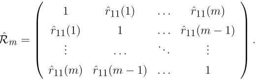
Peˇna and Rodriguez (2002) proposed a univariate portmanteau test statistic,

ˆ

Dm =n

1− |Rˆm | 1/m

, (1.9)

(19)

m+ 1,

ˆ Rm =

      

1 rˆ₁₁(1) . . . rˆ₁₁(m)

ˆ

r₁₁(1) 1 . . . ˆr₁₁(m−1)

..

. . . .. ...

ˆ

r₁₁(m) ˆr₁₁(m−1) . . . 1

       . (1.10)

Peˇna and Rodriguez(2002) derived the asymptotic distribution of ˆDm as gamma

using the standardized values of residual autocorrelations. Li (2004, §2.7) noted

several interesting interpretations for this statistic. It was shown in simulation

ex-periments (Peˇna and Rodriguez, 2002) that the ˆDm statistic had better power than

the test ofLjung and Box (1978) in many situations. One problem noted by Lin and

McLeod(2006) is that the test statistic ˆDm may not exist because, with the modified

version of the residual autocorrelations used, the residual autocorrelation sequence is

not always positive-definite or even non-negative definite. Furthermore, the size of

the test may not be accurate due to the asymptotic approximation (Li, 2004, p. 19).

To overcome these difficulties Lin and McLeod(2006) suggested using a Monte-Carlo

significance test and demonstrated that this approach provides a test with the correct

size and is often more powerful than the usual Ljung-Box test (Lin and McLeod,2006,

Table 6).

Peˇna and Rodriguez (2006) suggested taking the log of the (m+ 1)th root of the

determinant in Equation 1.10,

˜

Dm =−n(m+ 1)−1log|Rmˆ | (1.11)

and they derived a gamma distribution approximation for this test statistic.

In the portmanteau tests based on the asymptotic distribution (Ljung and Box,

1978; Peˇna and Rodriguez, 2002, 2006) not only is the size of the test inaccurate if

(20)

lags, is not large enough as well. The Monte-Carlo significance test approach does not

require any such assumption about m and has much better finite-sample properties

than tests based on the asymptotic distribution.

1.2 NEW MULTIVARIATE PORTMANTEAU TEST

The univariate residual autocorrelations in the Toeplitz matrix in Equation 1.10 are

replaced by, Rˆ_`, `= 1, . . . , m in Equation 1.3,

ˆ

Rm =

      

Ik Rˆ1 . . . Rˆm

ˆ

R₁0 _I_k . . . Rˆ_m₋₁

..

. . . .. ...

ˆ

R0_m Rˆ0_m₋₁ . . . _I_k

       , (1.12)

where _I_k = ˆR0. The proposed multivariate portmanteau test statistic is

Dm =−nlog|Rˆm|. (1.13)

From Hadamard’s inequality for the determinant of a positive definite matrix,

|Rˆm| ≤ 1. When there is no significant autocorrelation in the residuals, ˆR` =

Op(n−

1

2_{) so ˆ}_R_m _{is approximately block diagonal and hence} _|_Rˆ_m_{| ≈}_1.

On the other hand, when there is autocorrelation present, |Rˆm| will be expected

to be smaller than 1. To see this we repeatedly apply the formula for the determinant

of a partitioned matrix (Seber, 2008, §14.1),

|Rˆm|= m Y

`=1

|_I_k−Rˆ₍_`₎Rˆ−_`₋1₁Rˆ0₍_`₎ |, (1.14)

where ˆR₍_`₎= [ ˆR1 :· · ·: ˆR`] is the k-by-`kblock partitioned matrix. Then ˆΣ` =Ik−

ˆ

(21)

order`is fit toLˆ0aˆt using the previous` values (Reinsel,1997, Equation 3.15). Thus,

Equation 1.14 is a direct multivariate generalization of the well known univariate

decomposition of generalized variance into the product of the one-step ahead variances

of the linear minimum-mean-square error predictors (McLeod, 1977, p. 532),

|Rmˆ |= m Y

`=1 ˆ

σ2_`, (1.15)

where ˆσ_`2 is the mean-square error for a fitted linear predictor of order`. In this case,

R_`2 = 1−σˆ_`2, where R2_` is the square of the multiple correlation for the order ` linear

predictor, and so (Peˇna and Rodriguez,2002, Equation 7),

|Rˆm |= m Y

`=1

(1−R_`2). (1.16)

In the multivariate case,

ˆ

η_`2 = 1− |_I_k−Rˆ₍_`₎Rˆ−_`₋1₁Rˆ0₍_`₎| (1.17)

is the proportion of the generalized variance that is accounted for by a linear predictor

of order `. From Equations 1.14 and 1.17, the corresponding multivariate equivalent

of Equation 1.16 is

|Rˆm|= m Y

`=1

(1−ηˆ2_`). (1.18)

It follows from Equation 1.18 that |Rˆm|<1 and that the smaller the value of |Rˆm|,

the more strongly autocorrelated the normalized residuals, Lˆ0aˆt, are.

Using the Chitturi (1974) multivariate residual autocorrelations, Equation 1.6,

the correlation matrix corresponding to Equation 2.10, ˆR(m‡), is defined by the block

matrix with (i, j)-block, ˆR(_i₋‡)_j for i, j = 1, . . . , m+ 1. This matrix is not symmetric

(22)

Multivariate autocorrelations are often defined as in Equation1.5(Box et al.,2008,

Equation 14.1.2). Using this definition, the residual autocorrelation matrix may be

written,

ˆ

R(_`†)=Dˆ−1/2Γˆ_`Dˆ−1/2, (1.19)

whereDˆ−1/2 = diag (ˆγ₁−_,₁1/2(0), . . . ,γˆ_k,k−1/2(0)). The correlation matrix corresponding

to Equation 2.10 obtained by replacing ˆR_` by ˆR_`(†) may be denoted by ˆR(_`†) and the

corresponding generalized variance portmanteau statistic, |Rˆ(m†) |. A similar

decom-position as given in Equation1.18shows that small values|Rˆ(m†) |correspond to

posi-tive autocorrelation. On the other hand, when there is no autocorrelation present, the

off-block diagonal entries in the matrix ˆR(m†)areOp(n−1/2). So,|Rˆ(m†) |≈|Rˆ(₀†)|m+1.

When the innovation variance matrix,Γ0, has large off-diagonal elements,|Rˆ(₀†) |<1.

Hence again | Rˆ(m†) |=Op(rm) for some r ∈(0,1). So, in both cases, autocorrelation

or no autocorrelation, | Rˆ(_m†) | tends to be small provided the innovation covariance

matrix is not diagonal. Numerical experiments confirmed that the test using D(m†)

and Dm are essentially equivalent when Γ0 is diagonal but in the non-diagonal case,

D(m†) does not provide a useful test.

1.2.1 Asymptotic distribution and approximation

In this section, the asymptotic distribution forDm in Equation1.13is derived and an

approximation to this distribution is suggested. Since, as shown in Lin and McLeod

(2006, Figure 2) in the univariate case by simulation, the actual finite-sample

distri-bution for Dm converges slowly, the asymptotic distribution for Dm is not expected

to be of much use in diagnostic checking multivariate time series models unless n is

very large.

(23)

P∞

i=0ΨiBi and Π(B) = Θ(B)−1 = P∞i=0ΠiBi are matrix power series such that the elements Ψi and Πi converge exponentially to zero as i→ ∞. Define

G=       

G₀ 0 . . . 0

G1 G0 . . . 0

..

. ... . .. ...

G_m₋₁ G_m₋₂ . . . Gm−p

       , (1.20) and H =       

H0 0 . . . 0

H₁ H₀ . . . 0

..

. ... . .. ...

Hm−1 Hm−2 . . . Hm−q

       , (1.21)

where Gr=P∞i=0Γ0Ψ0i⊗Πr−i and Hr =Γ0⊗Πr.

Theorem 1. Assume that the model specified in Equation 1.1 has independent and

identically distributed innovations with mean zero and constant covariance matrix.

The model is fit to a series of length n using an n−1/2-consistent algorithm. After

obtaining the residuals defined in Equation1.3 and the test statistic, Dm, in Equation

1.13, Dm is asymptotically distributed as

k2m X

i=1

λ_iχ2₁_,i,

where χ2₁_,i, i = 1, . . . , k2m are independent χ2₁ random variables and λ1, . . . , λ_k2_m

are the eigenvalues of (_I_k2−Q)M, where M is k2m×k2m diagonal matrix

M =       

m_I_k2 O . . . O

O (m−1)_I_k2 . . . O

..

. ... . .. ...

O O . . . _I_k2

(24)

and

Q=X(X0W−1X)−1X0W−1 (1.23)

is an idempotent matrix with rank k2(p+q), X is defined as k2m×k2(p+q) matrix

(G−H), and W =_Im⊗Γ0 ⊗Γ0 is positive-definite symmetric.

Proof. From the decomposition in Equation 1.14, it follows that,

−nlog|Rˆm|=−n m X

`=1

log |_I_k−A_` |, (1.24)

where A_` = ˆR₍_`₎Rˆ−_`₋1₁Rˆ0₍_`₎. Using the fact that|_I_k−A_` |=Qk

i=1(1−λi(`)), where

0< λ_i(`)<1 are the eigenvalues of A_`, ` = 1, . . . , m,

−nlog|Rˆm|=−n m X

`=1 k X

i=1

log(1−λ_i(`)). (1.25)

Expanding log(1−λ_i(`)) =−P∞

r=1r−1λri(`) and tr (A`) = Pki=1λi(`),

Dm =n m X

`=1

tr (A_`) +Op(n−1). (1.26)

One can verify that

tr (A1) = tr ( ˆR01Rˆ1)

tr (A₂)≈ tr ( ˆR0₁Rˆ₁) + tr ( ˆR0₂Rˆ₂) ..

.

tr (Am)≈ tr ( ˆR01Rˆ1) +. . .+ tr ( ˆR0mRˆm),

(1.27)

so that,

Dm ≈n m X

`=1

(25)

Using the commutative property of trace,

Dm ≈n m X

`=1

(m−`+ 1) tr ( ˆΓ0_`Γˆ₀−1Γˆ_`Γˆ−₀1). (1.29)

It follows from Neudecker (1969, Equation 2.12),

Dm ≈n m X

`=1

(m−`+ 1)( vec ˆΓ_`)0( ˆΓ₀−1⊗Γˆ−₀1) vec ˆΓ_`,

=n( vec ˆΓ)0(_Im⊗Γˆ₀−1 ⊗Γˆ−₀1)M( vec ˆΓ),

(1.30)

where vec ˆΓ= ( vec ˆΓ₁. . . vec ˆΓm) is k2m×1 column vector and M is k2m×k2m

diagonal matrix defined in Equation 1.22.

Hosking (1980, Theorem 1) showed that

√

n vec ˆΓ∼N_k2_m(0,(I_k2_m−Q)W), (1.31)

whereW−1 can be replaced by a consistent estimator ˆW−1 =_Im⊗Γˆ−₀1⊗Γˆ−₀1, and

Qis the idempotent matrix of rank k2(p+q) in Equation 1.23.

From the theorem on quadratic forms given by Box (1954, Theorem 2.1), and

Equations 1.30, 1.31, the asymptotic distribution ofDm is given by,

Dm → k2m

X

i=1

λ_iχ2₁, (1.32)

where → stands for convergence in distribution as n→ ∞ and λ1, . . . , λ_k2_m are the

eigenvalues of (_I_k2_m−Q)M.

1.2.1.1 Approximation

The upper percentiles of the cumulative distribution function in Equation1.32 could

(26)

(2006, Table 2) showed that the convergence to the asymptotic distribution is very

slow. In the case of large-samples, an approximation based on Box (1954, Theorem

3.1) works well. Using this result, the test statistic in Equation 1.32 can be

approx-imated by aχ2_b, where a and b are chosen to make the first two moments agree with

those of exact distribution of Dm. Hence, a = Pλ2_i/Pλi and b = (Pλi)2/Pλ2i,

where,

k2m X

i=1

λ_i = tr [(_I_k2_m−Q)M],

k2m X

i=1

λ2_i = tr [(_I_k2_m−Q)M(I_k2_m−Q)M].

(1.33)

When p = q = 0, a = (2m+ 1)/3 and b = 1.5k2m(m+ 1)/(2m + 1). In the

VARMA (p, q) case, one degree of freedom is lost for each parameter so Dm is

ap-proximately distributed as aχ2_b, where

a= 2m+ 1

3 ,

b= 3k

2_m(m_{+ 1)}

2(2m+ 1) −k

2_(p₊_q).

(1.34)

1.2.2 Monte-Carlo significance test

Monte-Carlo significance tests, originally suggested by George Barnard (Barnard,

1963), are feasible for many small-sample problems (Marriott,1979) and with modern

computing facilities these types of tests are increasingly feasible for larger samples and

more complex problems (Dufour and Khalaf,2001). For a pure significance test with

no nuisance parameters, as is the case, for example, for simply testing a time series for

randomness, the accuracy of the Monte-Carlo procedure depends only on the number

of simulations (Dufour, 2006, Proposition 2.1).

(27)

and Dufour (2006, Proposition 5.1) has shown that, provided consistent estimators

are used, Monte-Carlo tests remain asymptotically valid. Since we assume n−1/2

-consistent estimators are used, the requirements for Dufour (2006, Proposition 5.1)

are met.

Simulations for Dm in the univariate case (Lin and McLeod, 2006, Table 3) as

well as our simulations for the multivariate case in Section 1.3.1, suggest the impact

of nuisance parameters is negligible. The p-value for all of the portmanteau test

statistics presented in this paper may be obtained using the Monte-Carlo method

outlined below. We use the statistic Dm in the description but ˜Qm could be used

instead.

Step 1: Set N, the number of simulations. Usually, N ← 1000 but smaller values

may be used if necessary. By choosingN large enough, an accurate estimate of

the p-value may be obtained.

Step 2: After fitting the model and obtaining the residuals, compute the

portman-teau test statistic for lag m or possibly a set of lags such as ` = 1, . . . , m,

where m ≥ 1. Typically m is chosen large enough to allow for possible

high-order autocorrelations. Denote the observed value of the test statistics by

D(_`o), ` = 1, . . . , m.

Step 3: For eachi= 1, . . . , N, simulate the fitted model, refit it, obtain the residuals

from this model, compute the test statistic,D(_`i), `= 1, . . . , m.

Step 4: For each `, `= 1, . . . , m, the estimated p-value is given by,

ˆ

p= #{D (i) ` ≥D

(o)

` , i= 1,2, . . . , N}+ 1

(28)

The approximate 95% margin of error for the p-value is, 1.96ppˆ(1−ˆp)/N.

The above algorithm is simply a restatement of the Monte-Carlo testing algorithm

given by Lin and McLeod (2006, §3) for the univariate case. Lin and McLeod (2006,

Table 3) demonstrate that the Monte-Carlo testing procedure has the correct size for

an AR (1) and this is verified for some VAR (1) models in Section 1.3.1.

Remark 1. In the Monte-Carlo test procedure it is assumed that the innovations

used in our simulations in Step 3 are normally distributed but any distribution with

constant covariance matrix could be used. In particular, using the empirical joint

distribution is equivalent to bootstrapping the multivariate residuals. Using

boot-strapped residuals is implemented in our software (Mahdi and McLeod, 2011).

Remark 2. A limitation of the Monte-Carlo diagnostic check is the assumption of

constant variance. Many financial time series exhibit conditional heteroscedasticity.

In practice this means that our test may overstate the significance level (Duchesne and

Lalancette, 2003). This means that when used for constructing a VAR or VARMA

model, the final fitted model may not be as parsimonious as a model developed using

a portmanteau test which takes into account conditional heteroscedasticity (Francq

and Ra¨ısi, 2007; Duchesne, 2006). Our Monte-Carlo portmanteau test can also be

used to test for the presence of multivariate conditional heteroscedasticity simply

by replacing the residuals by squared or absolute residuals. An illustration of this

procedure is given later in Section1.4.2.

Remark 3. Francq and Ra¨ısi (2007) discuss a more general asymptotic multivariate

portmanteau diagnostic test that is valid assuming only that the innovations are

uncorrelated. This test requires a large sample though.

Remark 4. Lin and McLeod (2008) discuss the Monte-Carlo portmanteau test for

(29)

(2008) for infinite-variance ARMA has been extended to the multivariate case as well

and is available in our R package (Mahdi and McLeod, 2011).

1.3 SIMULATION RESULTS

The purpose of our simulations is to demonstrate the improved power as well as the

correct size of the Monte-Carlo (MC) test usingDm. We also compare the empirical

Type 1 error rates for the aχ2_b-approximation discussed in Section 1.2.1.1.

1.3.1 Comparison of type 1 error rates

The empirical error rates have been evaluated under the Gaussian bivariate VAR (1)

process Zt =ΦiZt−1+at, i= 1, . . . ,4 for the portmanteau test statistic Dm using

the MC and aχ2_b-approximation to evaluate the p-value. The covariance matrix of

a_t has unit variances and covariance 1/2 and the coefficient matrices are taken from

Hosking (1980) and Li and McLeod (1981),

Φ₁ = 0.9 0.1 −0.6 0.4

!

,Φ₂ = −1.5 1.2 −0.9 0.5

!

,Φ₃ = 0.4 0.1

−1.0 0.5

!

,Φ₄ = 0.3 0.5 0.0 0.3

!

.

The empirical error 1% and 5% rates are shown in Table 1.1. For each entry in

Table 1.1, 103 simulations were done. The MC test also usedN = 103.

The 95% confidence interval assuming a 5% rejection rate for each test is (3.6,6.4).

At the 5% rejection rate, there are 17 entries outside this interval with the aχ2_b

ap-proximation and only one 1 with the Monte-Carlo test. In conclusion, size-distortion

with the Monte-Carlo test appears to be negligible but is sometimes present when the

aχ2_b approximation is used.

In Section 1.4, we found that there is a much larger discrepancy between the

(30)

α= 1% α= 5%

n= 100 n= 200 n= 500 n= 100 n= 200 n= 500

m aχ2_b MC aχ2_b MC aχ2_b MC aχ2_b MC aχ2_b MC aχ2_b MC

Φ1

5 1.2 0.8 1.2 0.9 1.0 0.7 5.9 4.6 5.1 4.7 4.8 4.8 10 1.2 0.7 1.0 0.8 0.8 0.9 5.2 4.5 4.4 5.2 3.7 4.2 15 1.3 0.7 1.1 0.7 0.8 0.9 5.7 5.4 4.5 4.4 3.6 3.8 20 1.6 0.7 1.1 0.7 0.8 0.9 6.8 5.8 4.8 4.0 3.8 3.8 25 2.0 0.8 1.2 0.7 0.9 0.8 7.8 4.9 5.3 4.1 4.0 4.0 30 2.5 1.1 1.4 0.7 0.9 0.8 9.0 4.8 5.8 3.7 4.4 4.1 Φ2

5 0.9 0.9 0.8 1.2 0.7 1.0 4.7 4.8 4.0 4.8 3.5 4.7 10 1.0 0.7 0.9 1.3 0.6 1.4 4.8 3.8 3.8 4.0 3.5 4.8 15 1.2 1.0 1.0 0.8 0.7 1.5 5.7 3.9 4.3 3.9 3.6 5.0 20 1.7 0.8 1.0 0.8 0.7 1.2 6.9 4.2 4.9 4.2 3.8 4.8 25 2.0 0.7 1.0 0.7 0.7 1.0 8.2 4.0 5.3 3.9 4.1 5.3 30 2.4 0.7 1.3 0.6 0.7 1.0 9.5 4.3 5.8 4.0 4.5 5.4 Φ3

5 0.7 0.9 0.9 1.2 0.6 1.0 4.0 4.6 3.6 5.7 3.2 5.2 10 1.0 0.7 0.8 1.5 0.7 0.8 4.5 4.8 3.8 6.5 3.1 5.3 15 1.1 0.9 0.8 0.8 0.6 1.0 5.1 4.2 4.1 6.3 3.3 5.1 20 1.5 0.9 0.9 0.7 0.7 1.3 6.6 4.3 4.6 6.2 3.6 5.2 25 1.9 0.9 1.0 0.7 0.8 1.0 7.7 4.5 5.3 5.4 4.0 5.3 30 2.3 0.8 1.2 0.8 0.8 1.3 9.0 4.2 5.9 5.5 4.3 5.0 Φ4

5 0.6 0.8 0.6 1.1 0.5 1.0 2.9 4.3 2.6 4.7 2.5 5.2 10 0.8 0.8 0.7 1.1 0.6 1.0 3.9 4.6 3.2 4.9 3.0 4.5 15 1.0 0.9 0.9 1.0 0.6 1.0 4.9 4.1 3.9 4.6 3.2 5.0 20 1.3 1.2 0.9 1.0 0.7 1.0 6.1 4.4 4.5 5.3 3.6 4.9 25 1.8 0.9 1.1 1.0 0.7 1.0 7.3 3.9 5.0 5.0 3.9 4.8 30 2.2 1.0 1.3 1.0 0.8 0.9 8.7 3.9 5.6 5.2 4.3 4.7

(31)

1.3.2 Power comparisons

Only Monte-Carlo significance tests are used to compare the empirical power of 1%

and 5% level tests with ˜Qm and Dm. Possible size-distortion sometimes makes power

comparisons between asymptotic tests and Monte-Carlo tests invalid. In our

compar-isons, VAR models are fitted to various multivariate models. The power of diagnostic

tests using Dm versus ˜Qm are compared using simulation. In all comparisons, the

p-values were evaluated using the Monte-Carlo (MC) method withN = 103. We

con-sider a VAR (1) model fitted to simulated data generated from eight VARMA models

selected from well-known textbooks as cited below.

Model 1

L¨utkepohl (2005, p. 17).

"

Z₁_,t

Z₂_,t

# − " 0.5 0.1 0.4 0.5 # "

Z₁_,t₋₁

Z₂_,t₋₁

# − " 0 0 0.3 0 # "

Z₁_,t₋₂

Z₂_,t₋₂

#

=

"

a₁_,t

a₂_,t

#

Γ₀ = 1.00 0.71 0.71 1.00

!

Model 2

Brockwell and Davis (1991, p. 428).

"

Z1,t

Z₂_,t

# − " 0.7 0 0 0.6 # "

Z1,t−1

Z₂_,t₋₁

#

=

"

a1,t

a₂_,t

# − " 0.5 0.6 −0.7 0.8 # "

a1,t−1

a₂_,t₋₁

#

Γ0 =

1.00 0.71

0.71 2.00

(32)

Model 3

Reinsel (1997, p. 81).

"

Z₁_,t

Z2,t

# − " 1.2 −0.5 0.6 0.3 # "

Z₁_,t₋₁

Z2,t−1

#

=

"

a₁_,t

a2,t

# − " −0.6 0.3 0.3 0.6 # "

a₁_,t₋₁

a2,t−1

#

Γ0 =

1.00 0.50

0.50 1.25

!

Model 4

Tsay [2005 2nd ed, p. 371].

"

Z₁_,t

Z₂_,t

# − " 0.8 −2 0 0 # "

Z₁_,t₋₁

Z₂_,t₋₁

#

=

"

a₁_,t

a₂_,t

# − " −0.5 0 0 0 # "

a₁_,t₋₁

a₂_,t₋₁

#

Γ₀ = 1.00 0.71 0.71 1.00

!

Model 5

Reinsel (1997, p. 25).

"

Z1,t

Z₂_,t

#

=

"

a1,t

a₂_,t

# − " 0.8 0.7 −0.4 0.6 # "

a1,t−1

a₂_,t₋₁

#

Γ₀ = 4 1 1 2

(33)

Model 6

Tsay [2005 2nd ed, p. 350].

"

Z₁_,t

Z2,t

#

=

"

a₁_,t

a2,t

# − " 0.2 0.3 −0.6 1.1 # "

a₁_,t₋₁

a2,t−1

#

Γ0 =

2 1

1 1

!

Model 7

L¨utkepohl (2005, p. 445).

"

Z₁_,t

Z₂_,t

# − " 0.5 0.1 0.4 0.5 # "

Z₁_,t₋₁

Z₂_,t₋₁

# − " 0 0 0.25 0 # "

Z₁_,t₋₂

Z₂_,t₋₂

#

=

"

a1,t

a₂_,t

# − " 0.6 0.2 0 0.3 # "

a1,t−1

a₂_,t₋₁

#

Γ₀ = 1.0 0.3 0.3 1.0

!

Model 8

(34)



  

Z1,t

Z₂_,t

Z3,t

    −    

0.4 0.3 −0.6

0.0 0.8 0.4

0.3 0.0 0.0

       

Z1,t−1

Z₂_,t₋₁

Z3,t−1

    =    

a1,t

a₂_,t

a3,t

    −    

0.7 0.0 0.0

0.1 0.2 0.0

−0.4 0.5 −0.1

       

a1,t−1

a₂_,t₋₁

a3,t−1



  

Γ0 =



  

1.0 0.5 0.4

0.5 1.0 0.7

0.4 0.7 1.0



  

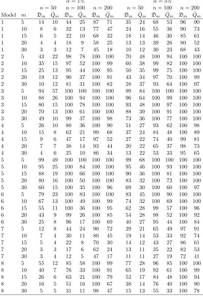
The power of the portmanteau statisticsDmand ˜Qmfor nominal 1% and 5% tests

using the MC test are shown in Table1.2. The power is evaluated for 104 simulations

for each parameter setting and N = 103 is used in the MC algorithm. It is clear

from Table 1.2 that the Dm test is often substantially more powerful than the ˜Qm.

Only whenn = 50 andm= 30 is the ˜Qm test more powerful and this only occurs for

(35)

α= 1% α= 5%

n= 50 n= 100 n= 200 n= 50 n= 100 n= 200 Model m D_m Q˜m Dm Q˜m Dm Q˜m Dm Q˜m Dm Q˜m Dm Q˜m

1 5 14 10 44 25 87 71 35 24 68 53 96 90

1 10 8 6 32 13 77 47 24 16 55 36 90 73

1 15 6 5 22 10 68 32 18 14 46 30 85 61

1 20 4 4 18 9 58 25 13 13 39 26 80 52

1 30 3 3 12 7 45 18 10 12 30 23 68 43

2 5 43 22 98 78 100 100 70 48 100 94 100 100 2 10 35 15 97 52 100 99 60 38 99 82 100 100 2 15 25 13 95 44 100 95 50 35 99 75 100 100 2 20 19 12 90 37 100 91 43 34 97 70 100 99 2 30 10 12 81 31 100 82 28 37 93 64 100 97 3 5 94 57 100 100 100 100 99 84 100 100 100 100 3 10 88 26 100 94 100 100 96 64 100 99 100 100 3 15 80 15 100 78 100 100 93 48 100 97 100 100 3 20 70 13 100 61 100 100 88 39 100 91 100 100 3 30 49 10 99 37 100 98 73 36 100 77 100 100

4 5 26 10 80 36 100 90 51 27 93 62 100 98

4 10 15 8 62 21 99 68 37 24 84 48 100 89

4 15 9 6 47 17 97 52 27 22 74 40 99 81

4 20 7 7 38 14 93 44 20 22 65 37 98 73

4 30 4 6 25 10 86 34 13 22 53 33 95 65

5 5 99 49 100 100 100 100 99 68 100 100 100 100 5 10 95 25 100 84 100 100 95 46 100 93 100 100 5 15 88 19 100 66 100 100 90 36 100 81 100 100 5 20 80 16 100 50 100 100 83 32 100 72 100 100 5 30 60 15 100 35 100 96 69 30 100 60 100 97 6 5 79 23 100 83 100 100 83 45 100 90 100 100 6 10 67 13 100 49 100 99 74 32 100 69 100 100 6 15 55 11 100 36 100 95 62 28 99 57 100 96

6 20 43 9 99 26 100 85 54 28 98 52 100 92

6 30 25 8 96 17 100 69 40 27 95 44 100 84

7 5 12 8 44 24 90 72 29 21 65 49 97 91

7 10 7 4 30 11 80 45 19 14 53 33 92 74

7 15 5 4 22 8 70 30 14 12 43 27 86 61

7 20 3 3 17 6 62 24 13 11 35 22 82 53

7 30 3 4 12 5 47 17 11 11 27 19 72 41

8 5 55 12 85 58 100 99 77 28 96 85 100 100

8 10 40 7 76 33 100 91 65 19 92 61 100 99

8 15 26 6 63 21 100 79 52 17 84 48 100 94

8 20 16 5 51 16 100 67 38 14 76 40 100 90

8 30 5 5 31 11 98 47 15 13 55 33 100 78

(36)

1.4 ILLUSTRATIVE APPLICATIONS

1.4.1 IBM and S&P index

Tsay (2010, Chapter 8) uses the portmanteau diagnostic test in constructing a VAR

model for the monthly log returns of IBM stock and the S&P 500 index for January

1926 to December 2008. So here, n = 996. Univariate analysis for both of these

series indicates the presence of conditional heteroscedasticity (Tsay, 2010, p. 408)

but for forecasting purposes, we may consider a VAR model rather than a more

complex VAR/GARCH model (Weiss,1984;Francq and Ra¨ısi,2007). The AIC selects

a VAR(5) model. We found that the BIC selects a VAR(1) model. Table1.3compares

the p-values for the portmanteau tests for the VAR(p) for p= 1,3,5.

These portmanteau tests suggest that the VAR(5) is adequate and that the VAR(1)

and VAR(3) both exhibit lack of fit. The VAR(4) is not shown but the results for

this model are similar to the VAR(3). As noted in Remark 2, the presence of

condi-tional heteroscedasticity means that the p-values in Table 1.3 are too small and this

implies that, possibly, a lower order model than the VAR(5) may be adequate. This

possibility could be investigated using the multivariate portmanteau test of Francq

and Ra¨ısi (2007).

Table 1.3 also shows that aχ2_b approximation for the p-value of Dm is inaccurate

whereas for ˜Qm the asymptotic approximation agrees quite well with the Monte-Carlo

result.

1.4.2 Investment, income and consumption time series

The trivariate quarterly time series, 1960–1982, of West German investment, income,

and consumption was discussed by L¨utkepohl (2005, §3.2.3). For this series, n = 92

(37)

VAR(1) VAR(3) VAR(5)

aχ2_b MC aχ2_b MC aχ2_b MC

m Dm Q˜m Dm Q˜m Dm Q˜m Dm Q˜m Dm Q˜m Dm Q˜m

5 0.2 * * * 10.4 0.6 1.7 0.6 NA NA 91.2 89.9

10 0.1 0.3 * 0.2 13.5 6.1 2.8 4.0 77.4 50.3 59.4 50.2

15 0.3 2.1 * 2.2 20.4 22.3 6.4 22.1 84.0 61.2 63.1 61.4

20 0.2 * * * 15.4 2.6 5.0 2.2 71.8 11.3 45.2 9.9

25 0.1 * * * 8.7 1.1 2.3 0.7 53.0 7.6 27.5 7.1

30 0.2 * * * 7.3 2.7 2.3 2.2 46.2 13.7 23.3 12.0

Table 1.3: IBM and S&P 500 Index Data. aχ2_b: approximation. MC: Monte-Carlo N = 103. NA: not applicable. The p-values are in percent. The ∗indicates a p-value less than 0.1%.

differences. Using the AIC, L¨utkepohl (2005, Table 4.5) selected a VAR (2) for this

data. Only lags m = 5,10,15 are used in the diagnostic checks since n is relatively

short. All diagnostic tests reject simple randomness, VAR (0). The Monte-Carlo tests

for VAR (1) suggests model inadequacy at lag 5. Table1.4 supports the choice of the

VAR (2) model.

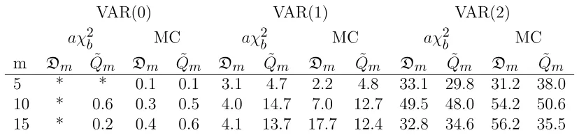
VAR(0) VAR(1) VAR(2)

aχ2_b MC aχ2_b MC aχ2_b MC

m Dm Q˜m Dm Q˜m Dm Q˜m Dm Q˜m Dm Q˜m Dm Q˜m

5 * * 0.1 0.1 3.1 4.7 2.2 4.8 33.1 29.8 31.2 38.0

10 * 0.6 0.3 0.5 4.0 14.7 7.0 12.7 49.5 48.0 54.2 50.6 15 * 0.2 0.4 0.6 4.1 13.7 17.7 12.4 32.8 34.6 56.2 35.5

Table 1.4: Trivariate West German Macroeconomic Series. aχ2_b: approximation. MC: Monte-Carlo using 103 replications. The p-values are in percent and∗ indicates a p-value less than 0.1%.

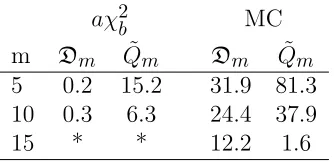
As pointed out in Remark 2, we may test for multivariate heteroscedasticity by

using the squared residuals and Table 1.5 gives the p-values with this test for the

(38)

approximation for ˜Qm are quite inaccurate. Based on the Monte-Carlo tests there is

little evidence to reject that null hypothesis of constant variance.

aχ2_b MC

m Dm Q˜m Dm Q˜m

5 0.2 15.2 31.9 81.3

10 0.3 6.3 24.4 37.9

15 * * 12.2 1.6

(39)

1.5 CONCLUDING REMARKS

Box et al.(2008) stress the importance of constructing an adequate and parsimonious

model in which the residuals pass a suitable portmanteau diagnostic check. In

fore-casting experiments with monthly riverflow time series, Noakes et al. (1985) found

that simply using a criterion such as the AIC or BIC may provide a model that either

does not pass a suitable diagnostic check for randomness of the residuals or that may

have more parameters than necessary. Monthly riverflow time series models chosen

with the fewest number of parameters that pass the portmanteau diagnostic check

for periodic autocorrelation (McLeod, 1994) tend to produce better one-step ahead

forecasts (Noakes et al.,1985). McLeod(1993) suggested formulating the principle of

parsimony as an optimization problem: minimize model complexity subject to model

adequacy. In any case, in the overall approach suggested many years ago and

pre-sented in their recent book (Box et al., 2008), portmanteau diagnostic checks play a

crucial role in constructing time series models.

In Section1.2.2, Remark 2, it was pointed out the Monte-Carlo test withDm may

also be useful in diagnostic checking for multivariate conditional heteroscedasticity

when used with squared or absolute residuals. This test is implemented in Mahdi

and McLeod (2011). There is an extensive literature on testing residuals in AR and

ARMA models for conditional heteroscedasticity (Ling and Li, 1997; Duchesne and

Lalancette,2003;Duchesne,2004;Rodr´ıguez and Ruiz,2005;Duchesne,2006;

Chabot-Hall and Duchesne,2008). The power study presented Section 1.3.2suggests that the

Dm with squared or absolute residuals may be useful. Peˇna and Rodriguez (2002)

also suggested that using squared-residuals with their generalized-variance

portman-teau test would outperform the usual diagnostic check (McLeod and Li,1983). Other

(40)

omnibus portmanteau test such as Dm or ˜Qm when these alternatives hold. For

ex-ample,Rodr´ıguez and Ruiz(2005) developed a diagnostic check for heteroscedasticity

for the case of small autocorrelations.

The multivariate portmanteau diagnostic test developed by Francq and Ra¨ısi

(2007) does not require independent and identically innovations but only uncorrelated

innovations. This test would be appropriate for the bivariate example in Section1.4.1.

Scripts for reproducing all tables in this paper are available with our freely

avail-able software (Mahdi and McLeod, 2011). This package can utilize multicore CPUs

often found in modern personal computers as well as a computer cluster or grid

(Schmidberger et al., 2009). On a modern eight core personal computer, the

com-putations for Tables 1.4 and 1.5 take about one minute. Table 1.3 takes about six

minutes due to the longer series length and increased number of lags. The simulations

(41)

REFERENCES

Barnard, G. A. (1963). Discussion of ”The spectral analysis of point processes” by M. S. Bartlett. Journal of the Royal Statistical Society, B 25, 264–296.

Box, G. (1954). Some theorems on quadratic forms applied in the study of analysis of variance problems, I. effect of inequality of variance in the one-way classification.

The Annals of Mathematical Statistics 25(2), 290–302.

Box, G. and Pierce, D. (1970). Distribution of residual autocorrelation in autoregressive-integrated moving average time series models. Journal of Ameri-can Statistical Association 65(332), 1509–1526.

Box G., Jenkins G., and Reinsel, G. C. (2008). Time Series Analysis: Forecasting and Control (4th ed.). New York: Wiley.

Brockwell, P. J. and Davis, R. A.(1991). Time series: Theory and Methods (2nd ed.). New York: Springer-Verlag.

Chabot-Hall, D. and Duchesne, P. (2008). Diagnostic checking of multivariate nonlin-ear time series models with martingale difference errors. Statistics and Probability Letters 78(8), 997–1005.

Chitturi, R. V. (1974). Distribution of residual autocorrelations in multiple autore-gressive schemes.Journal of the American Statistical Association 69(348), 928–934.

Chitturi, R. V. (1976). Distribution of multivariate white noise autocorrelations.

Journal of the American Statistical Association 71(353), 223–226.

Duchesne, P. (2004). On robust testing for conditional heteroscedasticity in time series models. Computational Statistics and Data Analysis 46, 227–256.

Duchesne, P. (2006). Testing for multivariate autoregressive conditional heteroskedas-ticity using wavelets. Computational Statistics and Data Analysis 51(353), 2142– 2163.

Duchesne, P. and Lalancette, S. (2003). On testing for multivariate ARCH effects in vector time series models. The Canadian Journal of Statistics 31(3), 275–292.

(42)

Dufour, J.-M. and Khalaf, L. (2001). Monte-Carlo test methods in econometrics. In B. Baltagi (Ed.),Companion to Theoretical Econometrics, Chapter 23, pp. 494–519. Oxford: Blackwell.

Francq, C. and Ra¨ısi, H. (2007). Multivariate portmanteau test for autoregressive models with uncorrelated but nonindependent errors.Journal of Time Series Anal-ysis 28(3), 454–470.

Hosking, J. R. M. (1980). The multivariate portmanteau statistic. Journal of Amer-ican Statistical Association 75(371), 602–607.

Hosking, J. R. M. (1981a). Equivalent forms of the multivariate portmanteau statistic.

Journal of the Royal Statistical Society, Series B 43(2), 261–262.

Hosking, J. R. M. (1981b). Lagrange-multiplier tests of multivariate time-series mod-els. Journal of the Royal Statistical Society. Series B (Methodological) 43(2), 219– 230.

Imhof, J. P.(1961). Computing the distribution of quadratic forms in normal variables.

Biometrika 48, 419–426.

Li, W. K. (2004). Diagnostic checks in time series. New York: Chapman and Hall/CRC.

Li, W. K. and McLeod, A. I. (1981). Distribution of the residual autocorrelation in multivariate arma time series models. Journal of the Royal Statistical Society, Series B 43(2), 231–239.

Lin, J.-W. and McLeod, A. I. (2006). Improved Peˇna-Rodr´ıguez portmanteau test.

Computational Statistics and Data Analysis 51(3), 1731–1738.

Lin, J.-W. and McLeod, A. I. (2008). Portmanteau tests for ARMA models with infinite variance. Journal of Time Series Analysis 29(3), 600–617.

Ling, S. and Li, W. K. (1997). Diagnostic checking of nonlinear multivariate time series with multivariate ARCH errors. Journal of Time Series Analysis 18(5), 447–464.

Ljung, G. M. and Box, G. E. P. (1978). On a measure of lack of fit in time series models. Biometrika 65, 297–303.

L¨utkepohl, H. (2005). New Introduction to multiple time series analysis. New York: Springer-Verlag.

(43)

Marriott, F. H. C. (1979). Barnard’s Monte Carlo tests: How many simulations?

Applied Statistics 28(1), 75–77.

McLeod, A. I. (1977). Improved Box-Jenkins estimators. Biometrika 64(3), pp. 531–534.

McLeod, A. I. (1993). Parsimony, model adequacy and periodic correlation in fore-casting time series. International Statistical Review 61(3), 387–393.

McLeod, A. I. (1994). Diagnostic checking periodic autoregression models with ap-plication. The Journal of Time Series Analysis 15(3), 221–233. Addendum, JTSA 16, 647–648.

McLeod, A. I. and Li, W. K. (1983). Diagnostic checking ARMA time series models using squared-residual autocorrelations. The Journal of Time Series Analysis 4, 269–273.

Neudecker, H. (1969). Some theorems on matrix differentiation with special reference to kronecker matrix products.Journal of American Statistical Association 64(327), 953–962.

Noakes, D. J., McLeod, A. I., and Hipel, K. W. (1985). Forecasting seasonal hydro-logical time series. The International Journal of Forecasting 1(1), 179–190.

Peˇna, D. and Rodr´ıguez, J. (2002). A powerful portmanteau test of lack of test for time series. Journal of American Statistical Association 97(458), 601–610.

Peˇna, D. and Rodr´ıguez, J. (2006). The log of the determinant of the autocorrelation matrix for testing goodness of fit in time series. Journal of Statistical Planning and Inference 8(136), 2706–2718.

Poskitt, D. S. and Tremayne, A. R. (1982). Diagnostic tests for multiple time series models. Annals of Statistics 6(1), 114–120.

Reinsel, G. C. (1997). Elements of multivariate time series analysis (2nd ed.). New York: Springer-Verlag.

Reinsel, G. C., Basu, S. and Yap, S. F. (1992). Maximum likelihood estimators in the multivariate autoregressive moving average model from a generalized least squares viewpoint. Journal of Time Series Analysis 13(2), 133–145.

(44)

Schmidberger, M., Morgan, M., Eddelbuettel, D., Yu, H., Tierney, L., and Mansmann, U. (2009). State of the art in parallel computing with R. Journal of Statistical Software 31(1), 1–27.

Seber, G. A. F. (2008). A matrix handbook for statisticians. New York: Wiley.

Tsay, R. S. (2010). Analysis of financial time series (3rd ed.). (2nd ed. 2005). New York: Wiley.

(45)

PORTMANTEAU TESTS FOR TIME SERIES MODELS: R PACKAGE portes

Chapter 2 PORTMANTEAU TESTS FOR TIME SERIES MODELS:

R PACKAGE portes

2.1 INTRODUCTION

The multivariate vector integrated autoregressive moving average, VARIMA (p,d, q),

model with mean vectorµand deterministic equationa+btfor ak-dimensional time

series Zt = (Z1,t, . . . , Zk,t)0 can be written as

Φ(B)D(B)(Zt−µ) = a+bt+Θ(B)et, (2.1)

whereΦ(B)=_I_k−Φ₁B− · · · −ΦpBp,Θ(B)=Ik−Θ1B− · · · −ΘqBq andIk is a

k×kidentity matrix,Φ_` = (φ_ij,`)_k_×_k, Θ_` = (θ_ij,`)_k_×_kare coefficient matrices, andB

is a backshift operator such asBjZt =Zt−j. D(B)= diag [(1−B)d1, . . . ,(1−B)dk]

is a diagonal k ×k matrix, where d = (d1, . . . , dk), di ≥ 0. This states that each

individual series Zi, i = 1, . . . , k is differenced di times to reduce to a stationary

VARMA (p, q) series. It is assumed that the VARMA model is stationary, invertible,

and identifiable (Reinsel, 1997; Box et al., 2008). The coefficients a and b represent

the constant drift and the deterministic time trend respectively and the white noise

process et = (e1,t, . . . , ek,t)0 is assumed to be uncorrelated in time with mean zero;

that is, E(et) = 0 and E(ete0_t₋_`) = Γ0δ`, where Γ0 is the k ×k positive definite

variance covariance matrix and δ_` is the usual Kronecker delta with unity at ` = 0

(46)

In univariate time series, i.e. when k = 1, the model in Equation 2.1 reduces to

be an integrated autoregressive moving average, ARIMA (p, d, q), model

φ(B)D(B)(Zt−µ) = a+bt+θ(B)et, (2.2)

whereaand b, are the drift and the trend terms respectively,φ(B) = 1−φ₁B− · · · −

φpBp, θ(B) = 1−θ1B− · · · −θqBq,D(B) = dis the differencing order, and et is the

white noise series with mean zero and variance σ2 (Hannan, 1969; Pfaff, 2006; Box

et al., 2008).

After fitting the ARIMA or VARIMA model using efficient estimators, the

resid-uals, ˆe_i,t where i = 1, . . . , k and t = 1, . . . , n can be obtained. We may then use

portmanteau goodness-of-fit test to test the adequacy of the fitted model by checking

whether the residuals are approximately white noise (Li,2004).

The most popular portmanteau tests that were introduced by Box and Pierce

(1970); Ljung and Box (1978); Hosking (1980); Li and McLeod (1981), with a new

portmanteau generalized variance test based on the determinant of the

standard-ized multivariate residual autocorrelations (Peˇna and Rodriguez,2002, 2006;Lin and

McLeod,2006; Mahdi and McLeod, 2011) are implemented in theR package portes.

In addition, the portmanteau tests for nonlinear structure in time series as proposed

byMcLeod and Li(1983) and for Fractional Gaussian Noise, FGN , stochastic model

(McLeod et al., 2007b) that possesses long memory, are also implemented in this

package. Adler et al.(1998) studied ARMA models with identical and independent

in-novations from stable distribution with infinite variances andLin and McLeod(2008)

developed a generalized variance portmanteau test for such models using Monte-Carlo

techniques and this test is also included in this package. Any other fitted model, such

(47)

proposed package (Cryer and Chan, 2010). Brief descriptions for different

portman-teau tests are given in Section 2.3.

The concern of using the portmanteau tests is that the accuracy of the asymptotic

distributions requires n and m large, where n denotes the length of the series and

m is the lag time value. The development of powerful computers, specially those

with multicore systems, in which the R packages Rmpi (Yu, 2002) and snow (

Tier-ney et al., 2011) work efficiently with parallel computing, has made Monte-Carlo

tests more affordable and recommended in such cases as simulation experiments show

that the Monte-Carlo tests are usually more accurate and powerful than asymptotic

distributions (Lin and McLeod, 2006; Mahdi and McLeod,2011).

In Sections 2.2 and 2.4 we describe the main function, portest(), with some

illustrative applications explaining the Monte-Carlo version of Peˇna and Rodriguez

(2002); Mahdi and McLeod (2011) portmanteau test with implementation to snow

package. This function can be used for testing whiteness of series as well as for

testing adequacy of fitted ARMA and VARMA models with finite or infinite variances,

GARCH effects, FGN models, or any other fitted model. To reproduce the results in

these sections, one should install the packagesfGarch,FGN,snow,TSA, andvars, on

a computer with a minimum requirement of dual core. These packages are available

from the ComprehensiveR Archive Network website, CRAN.

R> library("fGarch")

R> library("FGN")

R> library("snow")

R> library("vars")

The proposedR package portes is developed so one can simulate time series from

(48)

or infinite variance from stable distribution (see Section 2.5.2). The simulated data

may has a deterministic constant drift and time trend term with non-zero mean.

It can be used for testing stationarity and invertibility and for estimating stable

parameters of data from stable distribution. The package portes is available from

the Comprehensive R Archive Network, CRAN, at http://CRAN.R-project.org/

package=portes version 1.08 and can be installed in the usual ways and is ready to

use after typing

R> library("portes")

2.2 THE MAIN FUNCTION: portest

In this section we describe the main function, portest(). This function implements

the portmanteau test statistics as given in Box and Pierce (1970); Ljung and Box

(1978); Hosking (1980); Li and McLeod (1981); McLeod and Li (1983) with a new

portmanteau test statistic based on the determinant of the standardized univariate

or multivariate residual autocorrelations (Peˇna and Rodriguez, 2002, 2006; Lin and

McLeod,2006,2008;Mahdi and McLeod,2011). The p-values can be evaluated using

the Monte-Carlo techniques and the approximate asymptotic chi-square distribution.

The syntax of portest() is listed below:

portest(obj,lags=seq(5,30,5),order=0,test=c("gvtest","BoxPierce",

"LjungBox","Hosking","LiMcLeod"),MonteCarlo=TRUE,nslaves=1,

NREP=1000,InfiniteVarianceQ=FALSE,SquaredQ=FALSE,

(49)

2.2.1 Monte-Carlo goodness-of-fit test

The minimal required input of the function portest() is portest(obj). By

select-ing this argument, the generalized variance portmanteau statistic, gvtest(), that is

described in Section 2.3.5 will be implemented using the Monte-Carlo approach with

one thousand replications on a single CPU at lags 5, 10, 15, 20, 25, and 30.

As an illustrative example, consider the univariate series DEXCAUS. Data is

avail-able from ourRPackageportesand refer to daily Canada/US foreign exchanges rates

from January 04, 1971 to September 05, 1996. A complete description of the data can

be retrieved simply by typing ?DEXCAUSinR session. In this example, theportest()

function implements the Monte-Carlo version of the statistic gvtest with 103

repli-cations using a single CPU and test for randomness of returns. The results suggest

that the returnsseries behaves like random series. With respect to computer time,

the CPU time equals to 49.61 seconds to get the output of this example.

R> data("DEXCAUS")

R> returns <- log(DEXCAUS[-1]/DEXCAUS[-length(DEXCAUS)])

R> portest(returns)

Lags Statistic df p-value

5 5.726436 4.090909 0.2237762

10 12.002784 7.857143 0.1478521

15 16.798015 11.612903 0.1598402

20 20.847948 15.365854 0.1718282

25 23.805231 19.117647 0.2227772

30 27.248101 22.868852 0.2477522

For the Monte-Carlo significance test, the function portest()with an objectobj

Diagnostic Checking, Time Series and Regression

Scholarship@Western

Scholarship@Western

Diagnostic Checking, Time Series and Regression

Diagnostic Checking, Time Series and Regression

ABSTRACT

ACKNOWLEDGEMENTS

CONTENTS

LIST OF TABLES

LIST OF FIGURES

INTRODUCTION

REFERENCES

Chapter 1

IMPROVED MULTIVARIATE PORTMANTEAU TEST

1.1

INTRODUCTION

1.2

NEW MULTIVARIATE PORTMANTEAU TEST

1.3

SIMULATION RESULTS

1.4

ILLUSTRATIVE APPLICATIONS

1.5

CONCLUDING REMARKS

REFERENCES

Chapter 2

PORTMANTEAU TESTS FOR TIME SERIES MODELS:

R PACKAGE portes

2.1

INTRODUCTION

2.2

THE MAIN FUNCTION: portest