Linear Biases in AEGIS Keystream
Brice Minaud
ANSSI, 51, boulevard de la Tour-Maubourg, 75700 Paris 07 SP, France
Abstract. AEGIS is an authenticated cipher introduced at SAC 2013, which takes advantage of AES-NI instructions to reach outstanding speed in software. Like LEX, Fides, as well as many sponge-based designs, AEGIS leaks part of its inner state each round to form a keystream. In this paper, we investigate the existence of linear biases in this keystream. Our main result is a linear mask with bias 2−89 on the AEGIS-256 keystream. The resulting distinguisher can be exploited to recover bits of a partially known message encrypted 2188 times, regardless of the keys used. We also consider AEGIS-128, and find a surprising correlation between ciphertexts at roundsiand i+ 2, although the biases would require 2140 data to be detected. Due to their data requirements, neither attack threatens the practical security of the cipher.
Key words: Cryptanalysis, AEGIS, CAESAR
1
Introduction
Traditional block cipher-based encryption ensures the confidentiality of encrypted data: it is infeasible for anyone to decipher a message without knowledge of the secret encryption key. However there is a compelling need for ciphers achieving at once confidentiality and authenticity; that is, ciphers in-tegrating a form of integrity check guaranteeing that the encrypted message does originate from its purported sender. Any tampering of the data will result in its rejection by the deciphering algorithm. The CAESAR [cae13] authenticated cipher competition, sponsored by the National Institute of Stan-dards and Technology, crystallizes the community’s growing interest in this type of cipher. In March 2014, first round submissions were finalized and all entries were published online, awaiting analysis.
AEGIS [WP14] is a particularly notable candidate in this competition. Indeed, it takes full advan-tage of the new AES-NI instruction set in recent Intel and AMD processors to achieve unprecedented encryption speed in software, at around half a cycle per byte. Although AEGIS was first introduced only a year ago at SAC 2013, it has already inspired other encryption designs, including PAES [YWH+14] and Tiaoxin [Nik14]. The state update function at the core of AEGIS is simply the parallel applica-tion of a single AES round to a large state, followed by a shift and XOR. This exploits the pipeline implementation of AES-NI, which allows for the parallel computation of several AES rounds.
AEGIS, like many entries in the CAESAR competition, follows a model where a large inner state leaks essentially a portion of itself every round, which is then XOR-ed with the plaintext to form the ciphertext. Moreover, like most ciphers in this family, including all duplex-like constructions [BDPA12], it delays the insertion of a plaintext block into the inner state until after the corresponding ciphertext block has been output, in order for decryption to proceed in the same direction as encryption. As such, these ciphers are not proper stream ciphers, but form an interesting hybrid, where a single round behaves like a stream cipher.
In particular, assume we have a linear distinguisher on the ciphertext with known plaintext, which we call a keystream bias by analogy with stream ciphers. That is, we know that the sum of some specific bits of the ciphertext is biased towards 0 or 1, provided the corresponding plaintext has a known value. Then, because of the stream cipher-like behavior pointed out above, if only the last block of plaintext involved varies, and the rest remains fixed as before, the sum of ciphertext bits is biased towards 0 or 1 depending on the same sum on the plaintext.
that this does not require the same key be used. Indeed, this plaintext could be encrypted in entirely different sessions with different keys, as long as it is encrypted a sufficient number of times in total. This is very reminiscent of classic stream cipher attacks such as linear masking [CHJ02], as well as recent attacks on RC4 [ABP+13]. However, in the security analysis of AEGIS by its authors, as well as
many CAESAR submissions displaying similar stream cipher-like behavior, this type of attacks does not seem to be taken into account. This leaves open the question of how effective they might be, which we investigate for AEGIS.
Our contribution.
In this paper, we describe linear biases in the keystream of AEGIS-128 and AEGIS-256. As far as we know, this is the first cryptanalysis of AEGIS. These biases result from the surprising property that, although the inner state of AEGIS-128 (resp. AEGIS-256) is 5 (resp. 6) times the size of its output per round, the outputs of only 3 consecutive rounds are related. This is particularly striking in the case of AEGIS-128, where we show that the outputs of roundsiandi+ 2 are correlated.
However, the biases we find are quite small. In the case of AEGIS-256, we exhibit biases of 2−89 for a few linear masks, which would require 2188 data to be detected with good probability. This bias only requires a known plaintext to be encrypted repeatedly, with no assumption about the keys or nonces: in fact, the inner state before encryption is considered uniformly random. This distinguisher can also be exploited to recover information on a partially known plaintext encrypted 2188times. Due to the data requirements involved, our attack does not threaten the practical security of the cipher. For instance, restricting the attacker to not use more than 2128 data in total even for AEGIS-256, independently of the keys involved, would most likely prevent this type of attack entirely.
We also investigate linear biases of AEGIS-128, and find a bias of 2−77 between outputs of the cipher at roundsi and i+ 2. While this would require more than 2128 data, it is still worth noting, as this bias is vastly superior to any generic attack, considering the inner state is 640-bit long. In Appendix B, we investigate to what extent linear hull effects as well as multilinear techniques can be expected to reduce the data requirements. We find that around 2140data would likely still be required, showing that AEGIS-128 should be safe from our attack.
The first section provides a brief description of AEGIS-128 and AEGIS-256 encryption. In the second sction, we define linear biases, and study some linear biases linking substates of AEGIS. From there, we deduce biases in the keystream of AEGIS-128 and AEGIS-256. Finally, we show how these biases can be exploited to mount an attack.
1.1 Notations
For: n an integer
X an-bit vector
Y an-bit vector
α an-bit vector
Define: X⊕Y the bitwiseXORofX andY X&Y the bitwiseANDofX andY
α·X the scalar product ofαandX
|α| the Hamming weight ofα
2
Description of AEGIS-128 and AEGIS-256
2.1 AEGIS-128
AEGIS-128 takes as parameters a 128-bit key, a 128-bit nonce, and a tag length less than or equal to 128. It proceeds in several stages: initialization, where the 640-bit inner state is initialized using the key and nonce; processing of the authenticated data, where optional associated data is integrated into the state; encryption proper, where a variable-length plaintext is encrypted into a ciphertext of the same length; and finalization, which produces an authentication tag from the inner state. Hereafter we are only interested in the encryption step. A complete description of AEGIS can be found in [WP14]. The inner state of AEGIS-128 consists of five 128-bit substatesS0, . . . , S4. The plaintext is divided into 128-bit blocks mi,i ≥0, and processed in successive rounds. Let us denote by Si,0, . . . , Si,4 the values of the substates at roundi. For simplicity, we set i= 0 when encryption begins, setting aside the initialization step as well as the processing of authenticated data.
Then we have:
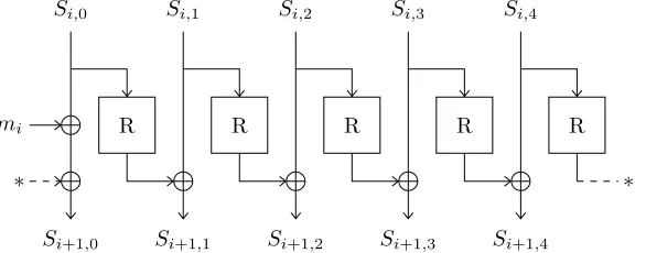
Si+1,0=Si,0⊕R(Si,4)⊕mi Si+1,1=Si,1⊕R(Si,0) Si+1,2=Si,2⊕R(Si,1) Si+1,3=Si,3⊕R(Si,2) Si+1,4=Si,4⊕R(Si,3)
where R denotes a single round of AES-128 [DR99], with no key addition. The state update function is depicted in Figure1.
Si,0
R
Si+1,0
Si,1
R
Si+1,1
Si,2
R
Si+1,2
Si,3
R
Si+1,3
Si,4
R
Si+1,4
* *
mi
Fig. 1. State update function of AEGIS-128.
Each round, the ciphertext is output as:
Ci=Si,1⊕Si,4⊕(Si,2&Si,3)⊕mi
2.2 AEGIS-256
AEGIS-256 takes as parameters a 256-bit key, a 256-bit nonce, and a tag length less than or equal to 128. The encryption step is very much the same as that of AEGIS-128, except the inner state consists of six rather than five 128-bit substatesSi,0, . . . , Si,5. The state update function may be written as:
Each round, the ciphertext is output as:
Ci=Si,1⊕Si,4⊕Si,5⊕(Si,2&Si,3)⊕mi
2.3 Security Claims
AEGIS-128 and AEGIS-256 claim a security level of respectively 128 and 256 bits for plaintext confi-dentiality (provided the attacker did not first break the integrity of the scheme, for which a security level of 128 bits is claimed in both cases–cf. [WP14], Section 3). There is no explicit bound on data requirements.
3
Preliminaries
3.1 Linear Biases and Weights
Since we will typically deal with probabilities very close to 1/2, it is convenient to define the bias of an event (as a shorcut for the bias of its probability):
Definition 1 (Bias).The biasof a an eventE is defined as:
Bias(E) = 2·Prob(E)−1
Definition 2 (Linear Bias).Consider a functionF :{0,1}n→ {0,1}n from nbits to nbits. Given an input mask α∈ {0,1}n and output mask β ∈ {0,1}n, the linear bias of F with masks α, β, is
defined as:
Bias(α·X⊕β·F(X) = 0)
withX uniformly random in{0,1}n.
Matsui’s classic piling-up lemma [Mat94] is commonly used to combine linear biases together.
Lemma 1 (Piling-up Lemma).Let X1, . . . , Xn be independent random binary variables. Then:
Bias(X1⊕ · · · ⊕Xn= 0) = Bias(X1= 0)× · · · ×Bias(Xn= 0)
In the rest of this article, biases will often be of the form±2−i, withian integer. This leads to the
following definitions:
Definition 3 (Weight of an Event). LetE be an event. The weight ofE is the positive real:
weight(E) =−log2 |Bias(E)|
If the bias is zero, we define the weight as∞.
Definition 4 (Weight of a Linear Bias).The weightof a linear bias is the weight of its bias. That is, with the previous notations:
weight(F, α, β) =−log2 |Bias(α·X⊕β·F(X) = 0)|
3.2 Linear Approximations of Bitwise AND
Forx,ytwo independent uniformly random binary variables, it can be easily checked that their product
x&y can be linearly approximated in four different ways: 0,x,y andx⊕y⊕1, each with probability 3/4. In particular, this implies the following lemma, which will be quite useful:
Lemma 2. Let X, Y be two independent uniformly random variables in {0,1}n, and α be a linear
mask in{0,1}n. Then:
weight α·(X&Y) = 0
= weight α·(X&Y ⊕X) = 0
= weight α·(X&Y ⊕Y) = 0
= weight α·(X&Y ⊕X⊕Y ⊕1) = 0
=|α|
where|α|denotes the Hamming weight of α. The biases are all positive.
4
Linear Biases for AEGIS-128 and AEGIS-256
4.1 Linear Biases between Substates
The output of AEGIS-128 at roundiisCi=Si,1⊕Si,4⊕(Si,2&Si,3)⊕mi. Using linear approximations
of & in the previous section, this can naturally be approximated as a sum of some substatesSi,j’s. As
a preliminary step towards exhibiting biases in the AEGIS-128 keystream, we point out some useful linear relations between substatesSi,j’s over three rounds.
Assume that at some round i, three consecutive plaintext blocks mi, mi+1, mi+2 are all-zeros. DenoteS0 =Si,0, . . . , S4 =Si,4. Then we can compute the value of substate 0 over the three rounds i,i+ 1,i+ 2 as:
Si,0=S0
Si+1,0=S0⊕R(S4)
Si+2,0=S0⊕R(S4) ⊕ R(S4⊕R(S3))
We are interested in the two differencesSi,0⊕Si+1,0andSi,0⊕Si+2,0. Let us begin with the first:
S0⊕Si+1,0= R(S4)
If we choose any linear maskα,β withw= weight(R, α, β), then by definition we have:
β·(S0⊕Si+1,0) =α·S4 with weight w (1)
Now consider the second difference:
Si+2,0⊕Si,0= R(S4) ⊕ R(S4⊕R(S3))
This is the derivative of R at point S4 with difference R(S3). Choose two linear masks β, γ with
w0= weight(R, β, γ). By the piling-up lemma, we get:
γ·(Si+2,0⊕Si,0) =β·S4 ⊕ β·(S4⊕R(S3)) with weight 2w0 (2) =β·R(S3)
Thus, the contribution ofS4cancels itself out.
Finally, we can combine the previous linear approximation of R alongα,β with (2) to get:
Note that the above approximations also hold forSi,1, . . . , Si,4 by shifting allSi,j’s involved along j modulo 5. Furthermore the same equalities hold for AEGIS-256 as well, except S3 and S4 in all three equations (1), (2), (3) becomeS4 andS5. The main takeaway in all cases is thatSi+1,j⊕Si,j is
correlated toSi,j−1, whileSi+2,j⊕Si,j is correlated toSi,j−2.
SB SR MC
SB SR MC
β β0 γ
α α0 β
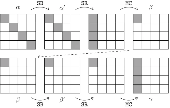
Fig. 2.Linear masks over two rounds of AES. Grey boxes denote active bytes.
In the end, we will want to chooseα,γso as to minimizew+ 2w0in (3). This involves considering
linear propagation over two rounds of AES. Due to the branching number of 5 of the AES construction [DR01], we will have at least 5 active S-boxes over these two rounds. Moreover, since we want to minimizew+2w0, the second round incurs twice the cost, so the optimal configuration would be to have
4 active S-boxes in the first round, and only one in the second round. This is easily achieved: choosing any linear masks at the input and output of a single S-box in the second round, then propagating the masks linearly will have the desired effect (cf. Figure2). In fact, there are enough degrees of freedom to pass all S-boxes with the optimal linear weight of 3. As a result, we getw= 4·3 = 12 and w0= 3,
sow+ 2w0= 18. Appendix A gives specific values forα,β,γ.
4.2 Biases for AEGIS-128
In this section, we will exhibit a linear bias between the output of AEGIS-128 at roundsi andi+ 2, assuming that the messagesmi,mi+1, mi+2 are all-zeros. Let us defineS0=Si,0, . . . , S4=Si,4.
Chooseα,β,γ as in the previous section. Recall that Ci =S1⊕S4⊕S2&S3. Using §3.2, we can approximateCi andCi+2as:
γ·Ci=γ·(S1 ⊕ S4 ⊕ S3) with weight |γ|
γ·Ci+2=γ·(Si+2,1 ⊕ Si+2,4 ⊕ Si+2,3) with weight |γ|
It follows from Equation (3) in the previous section that we have:
γ·(Ci⊕Ci+2) =α·(S4 ⊕ S2 ⊕ S1) with weight 3w+ 6w0+ 2|γ|
Now, observe thatCi may also be approximated as:
α·Ci=α·(S1 ⊕ S4 ⊕ S2) with weight |α|
We are now approximatingCibitwise in two different ways. However, as long asαandγhave disjoint
If we combine the last two equations together, we get:
(α⊕γ)·Ci⊕γ·Ci+2= 0 with weight 3w+ 6w0+|α|+ 2|γ|
This is an absolute bias on the AEGIS-128 keystream. Note that in order to simplify the presentation, we did not keep track of whether the bias is positive or negative; however, this is fixed and known.
The question now becomes how to choose α, γ so as to minimize the weight above. Details of this computation are provided in Appendix A. In the end, we obtain |α| = 5, |γ| = 9, with all S-boxes having optimal linear bias, hence w = 12, w0 = 3 as in the previous section. This yields
3w+ 6w0+|α|+ 2|γ|= 77.
4.3 Biases for AEGIS-256
Biases on the AEGIS-256 keystream are built essentially in the same way as for AEGIS-128, except the outputs of all three roundsi,i+ 1 andi+ 2 are necessary. Again, we assumemi=mi+1=mi+2= 0. Recall thatCi=S1⊕S4⊕S5⊕S2&S3.
We use the following approximations:
α·Ci =α·(S1 ⊕ S4 ⊕ S5) with weight|α|
β·Ci =β·(S1 ⊕ S4 ⊕ S5 ⊕ S2 ⊕ S3) with weight|β|
γ·Ci =γ·(S1 ⊕ S4 ⊕ S5 ⊕ S2) with weight|γ|
β·Ci+1=β·(Si+1,1 ⊕ Si+1,4 ⊕ Si+1,5 ⊕ Si+1,2 ⊕ Si+1,3) with weight|β| γ·Ci+2=γ·(Si+2,1 ⊕ Si+2,4 ⊕ Si+2,5 ⊕ Si+2,2) with weight|γ|
Using Equation (2) from §4.1, we have:
γ·(Ci⊕Ci+2) =β·(R(S5) ⊕ R(S2) ⊕ R(S3) ⊕ R(S0))
with weight 8w0+ 2|γ|
On the other hand:
β·(Ci⊕Ci+1) =β·(R(S0) ⊕ R(S3) ⊕ R(S4) ⊕ R(S1) ⊕ R(S2))
with weight 2|β|
Summing the last two equalities yields:
β·(Ci⊕Ci+1)⊕γ·(Ci⊕Ci+2) =β·(R(S1) ⊕ R(S4) ⊕ R(S5))
with weight 8w0+ 2|β|+ 2|γ|
Now it remains to use Equation (1) to pass through R and get:
β·(Ci⊕Ci+1)⊕γ·(Ci⊕Ci+2) =α·(S1 ⊕ S4 ⊕ S5)
with weight 3w+ 8w0+ 2|β|+ 2|γ|
Finally:
α·Ci⊕β·(Ci⊕Ci+1)⊕γ·(Ci⊕Ci+2) = 0
with weight 3w+ 8w0+|α|+ 2|β|+ 2|γ|
constraints. The same criterions are very fitting once again; the only difference is the newβterm, but with the previous choices|β| = 3, so it is nearly optimal as well. As a result, we have a weight of 3·12 + 8·3 + 5 + 2·3 + 2·9 = 89.
Intuition. How the previous linear approximations were chosen so as to cancel each other out, and perhaps more importantly what made such a choice possible, may not be immediately apparent from the description of the linear characteristic itself. As a result, it may be useful to provide some intuition.
We know thatSj⊕Si+1,j = R(Sj−1). From Eq. (2), Sj⊕Si+2,j = R(Sj−1)⊕R(Sj−1⊕R(Sj−2))
is linearly correlated to R(Sj−2), with the contribution ofSj−1 cancelling itself out; so we may write
Sj⊕Si+2,j = D(R(Sj−2)), where D is a purely formal notation to indicate an expression that is linearly
correlated to the input of D.
On the other hand, if we approximate the & operation in Ci and Ci+1 linearly along the same mask, and add them together, we can ensure that everySi+1,j is matched with the correspondingSj,
so as a result we can roughly write:
Ci+1⊕Ci≈ R(S0)⊕ [R(S1)]⊕ [R(S2)]⊕ R(S3)⊕ R(S4)
where the brackets denote a term that comes from a & operation and thus may be omitted at will by §3.2.
The same reasoning holds forCi+2; and in the end we have:
Ci≈ S1⊕ [S2]⊕ [S3]⊕ S4⊕ S5
Ci+1⊕Ci≈ R(S0)⊕ [R(S1)]⊕ [R(S2)]⊕ R(S3)⊕ R(S4)
Ci+2⊕Ci≈ [D(R(S0))]⊕ [D(R(S1))]⊕ D(R(S2))⊕ D(R(S3))⊕ D(R(S5))
Now take the characteristic α −R→ β −R→ γ from the previous section, which is also a character-istic α −R→ β −→D γ as can be seen in §4.1, Eq. (2). If the characteristics hold, this tells us that
α·Sk = β ·R(Sk) = γ ·D(R(Sk)). Hence, if we approximate the first line along α, the second
along β, and the third along γ, if the linear characteristics hold and we add up everything, any two terms in the same column will cancel each other out. So the question becomes simply how to make an appropriate choice for each bracket in the equations above so that there is 0 or 2 terms in each column. This is exactly what we do in order to construct our linear characteristic, namely:
Ci≈ S1⊕ S4⊕ S5
Ci+1⊕Ci≈ R(S0)⊕ R(S1)⊕ R(S2)⊕ R(S3)⊕ R(S4)
Ci+2⊕Ci≈ D(R(S0))⊕ D(R(S2))⊕ D(R(S3))⊕ D(R(S5))
If we look at AEGIS-128 from the same perspective, we can write:
Ci≈ S1⊕ [S2]⊕ [S3]⊕ S4
Ci+1⊕Ci≈ R(S0)⊕ [R(S1)]⊕ [R(S2)]⊕ R(S3)
Ci+2⊕Ci≈ [D(R(S0))]⊕ [D(R(S1))]⊕ D(R(S2))⊕ D(R(S4))
After removing the second line entirely, the approximation we made is:
Ci≈ S1⊕ S2⊕ S4
Ci+2⊕Ci≈ D(R(S1))⊕ D(R(S2))⊕ D(R(S4))
4.4 Exploiting the Keystream Biases
In the previous two sections, we have assumed that at some roundi, three consecutive plaintextsmi, mi+1,mi+2 are all-zeros. From there, we have shown the existence of an absolute bias of the form:
In other words, we have built a distinguisher on the AEGIS keystream. However, if we no longer assume
mi+2 = 0, then at roundi+ 2, the only difference in the output of the cipher is that mi+2 isXOR-ed into the ciphertextCi+2. As a result, we have:
Bias(α·Ci⊕β·Ci+1⊕γ·Ci+2⊕γ·mi+2⊕b= 0) = 2−w
Thus, the observable valueα·Ci⊕β·Ci+1⊕γ·Ci+2 directly leaks information aboutγ·mi+2.
This leads to the following attack scenario. Assume the same three consecutive plaintext blocks 0, 0,mare encrypted 22w times in total, independently of the keys and nonces used. Then an attacker
having access to that data would deduce the value ofγ·mwith good probability, just by counting the occurences of the eventα·Ci⊕β·Ci+1⊕γ·Ci+2= 0 on the fly. However, the data requirements make this attack impractical, since 2154and 2188 encryptions would be required respectively for AEGIS-128 and AEGIS-256 in order to exploit a single bias (as opposed to a multilinear approach). In Appendix B, we try to capture linear propagation in AEGIS-128 more accurately, in order to evaluate to what extent data requirements could be lowered; we conclude that AEGIS-128 seems to resist straightforward improvements of our attack, as 2140 data is still required.
5
Conclusion
In this article, we have constructed linear biases in the keystream of AEGIS-128 and AEGIS-256. These biases stem from dependencies between surprisingly few consecutive rounds: for AEGIS-128, linear biases exist between the outputs of roundsiandi+ 2; while for AEGIS-256, three consecutive rounds are enough. Our main result is the construction of a linear mask with bias 2−89on the keystream of AEGIS-256. This bias can be exploited to recover bits of information on a partially known plaintext encrypted 2188times, regardless of the keys involved. While the biases remain too low to be a threat in practice, they are vastly superior to any generic attack, and point out an unexpected property in the keystream of AEGIS.
Acknowledgments
The author would like to thank all members of the ANSSI cryptography laboratory, especially Thomas Fuhr and Henri Gilbert, for their valuable comments and insights on this article.
References
ABP+13. N. AlFardan, D. J. Bernstein, K. G. Paterson, B. Poettering, and J. Schuldt. On the security of RC4 in TLS. In USENIX Security Symposium (2013), Presented at FSE 2013 as an invited talk by Daniel J. Bernstein, available athttp://www.isg.rhul.ac.uk/tls/, 2013.
BDPA12. Guido Bertoni, Joan Daemen, Michal Peeters, and Gilles Assche. Duplexing the sponge: Single-pass authenticated encryption and other applications. In Ali Miri and Serge Vaudenay, editors,Selected Areas in Cryptography, volume 7118 ofLecture Notes in Computer Science, pages 320–337. Springer Berlin Heidelberg, 2012.
cae13. CAESAR– Competition for Authenticated Encryption: Security, Applicability, and Robustness. General secretary Daniel J. Bernstein, information available athttp://competitions.cr.yp.to/ caesar.html, 2013.
CHJ02. Don Coppersmith, Shai Halevi, and Charanjit Jutla. Cryptanalysis of stream ciphers with linear masking. In Moti Yung, editor,Advances in Cryptology CRYPTO 2002, volume 2442 ofLecture Notes in Computer Science, pages 515–532. Springer Berlin Heidelberg, 2002.
DR99. Joan Daemen and Vincent Rijmen. AES proposal: Rijndael. Advanced Encryption Standard submission, available athttp://jda.noekeon.org/, 1999.
Mat94. Mitsuru Matsui. Linear cryptanalysis method for des cipher. In Tor Helleseth, editor,Advances in Cryptology EUROCRYPT 93, volume 765 ofLecture Notes in Computer Science, pages 386–397. Springer Berlin Heidelberg, 1994.
Nik14. Ivica Nikoli´c. Tiaoxin–346. CAESAR submission, http://competitions.cr.yp.to/round1/ tiaoxinv1.pdf, 2014.
WP14. Hongjun Wu and Bart Preneel. AEGIS: A fast authenticated encryption algorithm. CAESAR submission, updated from Cryptology ePrint Archive Report 2013/695, updated from SAC 2013 version,http://competitions.cr.yp.to/round1/aegisv1.pdf, 2014.
Appendix A: Values of
α
,
β
,
γ
Consider the situation depicted on Figure 3, where the linear characteristic α → β → γ spans two rounds of AES (without key addition). We are trying to minimize|α|+ 2|γ|, while passing all S-boxes with optimal linear probability.
SB SR MC
SB SR MC
β β0 γ
α α0 β
Fig. 3.Linear masks over two rounds of AES. Grey boxes denote active bytes.
First, we look for β0 minimizing |γ|. With little-endian hexadecimal notations, it turns out only
one valueβ0 =0ereaches the minimum with |γ|= 9 (γ equals f, 8, c, 5 along one column). For
this value, five choices ofβ allow us to pass the S-box with weight 3:β =09, 31,38, c8, orf9. For each of these values, we computeα0, then look for the minimal size ofαsuch that all four S-boxes are
passed with optimal probability. We find|α|= 5, forβ=38(αequals4, 3, 2, 2along the diagonal). Observe that|α| is at least 4 since it has to span 4 S-boxes. Since we followed the only way to have |γ| = 9, which is optimal;|α|is within 1 of being optimal; and we are trying to minimize |α|+ 2|γ|, we have found the unique optimal choice.
More accurately, it is the unique optimal choice once we have fixed our choice for the active S-box in the second round. In fact, we could choose any one of the other 15 S-boxes, and use the exact same values of linear masksβ,β0 at the entrance of that S-box (namely, 38and0e). Indeed, the circulant
nature of the AESMixColumsmatrix means that a given mask at the input (resp. output) of one S-box will propagate to a permutation of the same masks at the output (resp. input) of the previous (resp. next) layer of S-boxes, and hence in our case will yield the same sizes forαandγ. Thus there are 16 choices forα,γwith identical properties for our purpose; one per choice of active S-box in the middle round.
Appendix B: Refined Linear Model of AEGIS-128
It so happens that for AEGIS-128, there is a fairly elegant way of simultaneously taking into account many of the effects listed above. In our previous analysis, we used standard linear cryptanalysis techniques to follow the propagation of a bias along a few AES-based transformations. This amounts to modelling the transformations in a certain way, materialized by independence assumptions. However in the case of AEGIS-128, large parts of the transformations can be computed with complete accuracy by looking at byte distributions, without the need to model anything.
If we recap the previous analysis in§4.2, we approximateCiandCi⊕Ci+2linearly, and from there we obtain the following two sums:
S1 ⊕ S2 ⊕ S4
and: R(S2)⊕R(S2⊕R(S1))⊕R(S3)⊕R(S3⊕R(S2))⊕R(S0)⊕R(S0⊕R(S4)) = D(R(S1)) ⊕ D(R(S2)) ⊕ D(R(S4))
where D is a purely formal notation denoting the fact that its input and output are linearly correlated (cf.§4.1); then we use the fact thatX and D(R(X)) are correlated. More precisely, we first relateX
to R(X), then R(X) to D(R(X)). Thus the propagation is decomposed in two steps, which we can picture as:
S1⊕S2⊕S4 → R(S1)⊕R(S2)⊕R(S4) → D(R(S1))⊕D(R(S2))⊕D(R(S4))
So our propagation “factors” through the value R(S1)⊕R(S2)⊕R(S4): that is to say, all information we had onS1⊕S2⊕S4 is first translated as information on R(S1)⊕R(S2)⊕R(S4); after which only information on R(S1)⊕R(S2)⊕R(S4) is used to deduce information on D(R(S1))⊕D(R(S2))⊕D(R(S4)). Moreover, with our linear masks, only a single S-box is active in R(S1)⊕R(S2)⊕R(S4), so actually the whole propagation factors through the value of R(S1)⊕R(S2)⊕R(S4) on a single byte.
The idea for our new model is that we are going to compute the actual distribution of R(S1)⊕ R(S2)⊕R(S4) on one byte from the knowledge ofCi=S1⊕S2&S3⊕S4. Then we are going to use this full distribution, rather than a single linear mask, to compute a distribution ofSi+2,3⊕S3 ⊕ Si+2,4⊕
S4 ⊕ Si+2,1⊕S1, which is our linear approximation ofCi⊕Ci+2along a linear maskγ. Thus we hope to compute the bias ofγ·(Ci⊕Ci+2) more accurately. A good motivation for this model is that the
two steps above: linking knowledge of Ci to the distribution of R(S1)⊕R(S2)⊕R(S4) on one byte;
and then the distribution of R(S1)⊕R(S2)⊕R(S4) on one byte to the bias of the linear approximation ofγ·(Ci⊕Ci+2), can be computed with perfect precision within complexity at most 232, as we show
below. Hence the only loss of precision results from “factoring” through R(S1)⊕R(S2)⊕R(S4); but as we saw in the previous paragraph, we were already making this approximation when we used standard linear characteristic techniques.
Thus, assume we know some specific value for Ci = S1⊕S2&S3 ⊕S4. Then we can actually compute the distribution of a single byte of R(S1)⊕R(S2)⊕R(S4) with full precision. Indeed, if we denote bySBtheSubByteslayer of AES, fromS1⊕S2&S3⊕S4 we can compute the distribution of SB(S1)⊕SB(S2)⊕SB(S4) in an exact manner, since each byte depends only on the valueS1, S2, S3, S4 on the same byte; so we need only guess 4 bytes simultaneously.
From there, we can also compute the distribution of R(S1)⊕R(S2)⊕R(S4) on a single byte exactly, since it is simply the independent sum of the previous byte distributions through the MixColumns matrix. Moreover, in the end, this distribution depends on only 16 bytes in total, which is 128 bits, so we can simply count how many choices lead to a specific value using a 128-bit integer, and the resulting distribution is prefectly precise. Thus, from knowledge of Ci = S1⊕S2&S3 ⊕S4, it is possible to compute the distribution of R(S1)⊕R(S2)⊕R(S4) on one byte with full precision.
Now for the second step of the propagation, we want to compute the distribution of the following value (i.e. the linear approximation ofCi⊕Ci+2 along the maskγ):
Si+2,3⊕S3 ⊕ Si+2,4⊕S4 ⊕ Si+2,1⊕S1
from the known distribution of:
R(S1)⊕R(S2)⊕R(S4)
More precisely, we are interested in the distribution of the first value beforeMixColumns(which is the last operation applied to each component), on a single byte, so R reduces to one S-box layer (and a permutation of the bytes).
At first sight, it suffices to guess the values of all R(Si)’s on this one byte. This only involves
guessing 5 bytes, requiring 240 operations, which is reasonable. However a better algorithm is possible by observing that the contribution ofS0andS4is independent from the rest on both sides. As a result, it suffices to compute these two distributions separately, then add them together:
R(S1)⊕R(S2)→R(S2)⊕R(S2⊕R(S1)) ⊕ R(S3)⊕R(S3⊕R(S2)) R(S4)→R(S0)⊕(S0⊕R(S4))
Thus the complexity drops down to 232 operations.
The end result is that for a fixed value ofCi=S1⊕S2&S3⊕S4, we can compute the distribution of R(S1)⊕R(S2)⊕R(S4) on one byte without any approximation. Then from this distribution, we can compute the distribution of one byte of the linear approximation ofCi⊕Ci+2beforeMixColumns, which is what we measure fromCi⊕Ci+2using our linear masks, modulo the cost of the linear approximation alongγ, which is 2|γ|.
We implemented this model, and results correlate fairly well with our previous anaysis. In particular, we recover the fact that the values ofβ0 we chose yields the strongest bias, although one other value seems as strong (namely12), which is not too surprising since it is one of the two second-best candidates as far as minimizing|γ|. The main difference is that we find a bias close to 2−72when we fixC
ito some
random value and measureγ·(Ci⊕Ci+2) according to our model, rather than 2−77 when we used
pure linear masking. We surmise this is mostly due to more information being taken into account at the input, resulting overall in more information at the output; although both steps of the new model behave slightly better than expected.