Mathematical Modeling of Impact of Possible Shock Dynamic
Loads on the Modern Composite Materials
Eugenе Sosenushkin1,*, Oksana Ivanova1, Elena Yanovskaya1, and Yuliya Vinogradova1 1
Moscow State Technological University "STANKIN", RU-127055, Moscow, Russia
Abstract. In this paper, we study the dynamic processes in materials reinforced with fibers, that can be represented as composite rods. There has been developed a mathematical model of wave propagation under the impact of a shock pulse in semi-infinite composite rods. It is believed that the considered composite rod consists of two layers formed by simpler rods of different isotropic materials with different mechanical properties. The cross sections of such rods are considered to be constant and identical. When such composite materials are impacted by dynamic loads, a significant part of the energy is dissipated due to the presence of friction forces between the contact surfaces of the rods. In this regard, we study the propagation of waves in an elastic fiber-rod, the layers of which interact according to Coulomb law of dry friction. The case of instantaneous excitation of rods by step pulses is investigated. The blow is applied to a rod made of a harder material. In the absence of slippage, the friction force gets a value not exceeding the absolute value of the limit. In the absence of slippage, the friction force takes a value not exceeding the absolute value of the limit. Let us consider the value of the friction force constant. Normal stresses and velocities satisfy the equations of motion and Hooke's law. The problem statement results in the solution of inhomogeneous wave equations by the method of characteristics in different domains, which are the lines of discontinuities of the solution. Solutions are found in all constructed domains. On the basis of the analysis of the obtained solution, qualitative conclusions are made and curves are constructed according to the obtained ratios. From the found analytical solution of the problem it is possible to obtain ratios for stresses and strain rates in composite rods and composite materials.
1 Introduction
Composites [1] in which the components are typically arranged at a certain frequency are of interest because of their ability to attenuate shock pulses [2]. The extreme complexity of the interaction of waves in the propagation of the shock pulse in the real composite material leads to the fact that modern theoretical methods of investigation of this problem are limited to strongly idealized models [3].
Modern pipeline transport systems are becoming increasingly in higher demand due to growing economic competition. Nowadays, pipelines may be located not just underground, where they may be subject to seismic shocks, but also in more aggressive and corrosive environments, for example, sea water. This necessitates the development of new materials and their mathematical models. The new mathematical models must take into account wide variety of materials used and complicated interactions between layers that form a composite material. The developers must consider the effects of friction conditions between layers, sliding of layers with respect to each other at macro-, micro, and nano-levels, and other intricate layer interaction effects while projecting and synthesizing new composite materials. Modeling of such materials allows reaching the increased dependability and service life of new
technological systems, including pipeline transport systems. [4,5].
In this work , a mathematical model of dynamic processes in materials reinforced with fibers, which are e represented by composite rods, has been developed.. When such materials are subject to dynamic loads, a significant portion of energy is dissipated due to friction forces between the contact surfaces of the rods. In this regards, , the propagation of waves in the elastic fiber-rod, layers of which interact according to the law of dry friction of the Coulomb [6-8], is consideredA semi-pointed composite rod consisting of two layers is examined. Each of the layers is considered to be an elastic rod of constant cross-section S. Part of the surfaces of these rods with perimeters of normal cross sections L interact with each other according to the law of dry friction of Coulomb. In the case when there is a slip between the rods, the tangential stresses on the side surface will be equal to fN where N is the lateral pressure on the rod and f is the coefficient of friction between the materials of the rods.
In the case, when there exist a relative movement between the rods on their surfaces, the limit friction force will act, the absolute value of which per unit length of the rods in the case of dry friction, is equal to
fLN
force assumes a certain value not exceeding the absolute limit [10].
2 Equations and mathematics
Let us consider two resilient rods interacting with each other according to the law of dry friction. We believe that for the first rod the Young's modulus has a meaning and density for the second one - and
ρ
2 Longitudinal elastic waves that propagate in the rodshave respective velocities and
Let us assume that , and place
the origin at the impact end of the second rod and point the x-axis along the rod (see Fig. 1)
Fig. 1. The settlement scheme.
The normal stresses in the rods
σ
1,
σ
2 and the speeds of their sectionsυ
1andυ
2 satisfy a system of equations composed of the equations of motion and Hooke's law in a differential form:;
1 1 1
q
t
x
χ
υ
ρ
σ
+
∂
∂
=
∂
∂
;
1 1
x
E
t
∂
∂
=
∂
∂
σ
υ
(1)
;
2 2
2
q
t
x
χ
υ
ρ
σ
−
∂
∂
=
∂
∂
;
2 2
x
E
t
∂
∂
=
∂
∂
σ
υ
(2)
.
S
fLN
q
=
The value
χ
=
sign
[
υ
1−
υ
2]
in the case of motion and in the case of rest takes any value between -1 and +1.The systems of equations (1) and (2) can be reduced to non-uniform wave equations.
In order to find a general solution to the non-uniform wave equation, it is necessary to use relationships along the characteristics of this equation.
Characteristics of non-uniform wave equations are lines:
dt
a
dx
=
±
1 anddx
=
±
a
2dt
.
A discontinuity in the solution extends along these lines.
Along the characteristics there are relations:
0
1 1
1
+
=
+
±
d
σ
a
ρ
d
υ
a
χ
qdt
(for the first rod);0
2 2
2
+
=
+
±
d
σ
a
ρ
d
υ
a
χ
qdt
(for the secondrod);
The solution to the Cauchy problem is sought in the form:
for the first rod:
(
)
(
)
;
2
1 1 1 1 11
a
f
a
t
x
a
a
t
x
qt
+
−
+
+
−
=
ϕ
ρ
χ
υ
(
)
(
)
,
2
1 1 1 11
E
f
a
t
x
E
a
t
x
qx
+
+
−
−
=
χ
ϕ
σ
(3)for the second rod:
(
)
(
)
;
2
2 2 2 2 22
a
f
a
t
x
a
a
t
x
qt
+
+
−
+
−
=
ϕ
ρ
χ
υ
(
)
(
)
.
2
2 2 2 22
E
f
a
t
x
E
a
t
x
qx
+
+
−
−
=
χ
ϕ
δ
(4)Problem statement.
Normal stress
σ
2 and velocityυ
2 of the rod which is subjected to shock satisfy the system (2).At time
t
=
0
all sections of the rod, except for0
=
x
, we consider stationary and undisturbed, i.e.0
=
=
υ
σ
,ift
=
0
andx
>
0
.
(5) At the end of the rod which is subject to an impact (x
=
0
), there is a condition:.
0
σ
σ −
=
(6) The area of motion from the area of rest in the task in question, at least to some extent, is determined by the characteristic ofx
=
a
2t
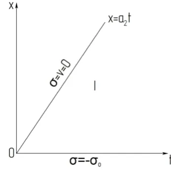
(fig. 2). The solution in the area (denoted by I) is sought as in the from (4) by the characteristic method.Fig. 2. The area of motion from rest point. 1
E
ρ
1;
E
21 1
1
ρ
E
a
=
.
2 2
2
ρ
E
The leading edge of the perturbation in the rod begins to spread as a shock. The condition for saving the movement quantity on the characteristic
x
=
a
2t
has the form
[ ]
σ
+
a
2ρ
2[ ]
υ
=
0
.
With regard to condition (5) this equation can be rewritten as:
0
2
2
=
+
ρ
υ
σ
a
ifx
=
a
2t
.
(7) From conditions (5) and (7) we find a solution in the area I for the second rod, considering thatχ
=
−
1
:
−
=
+
−
=
0 0 2
2
2
σ
σ
υ
ρ
υ
qx
qt
(8)
where
.
2 2
0
0
ρ
σ
υ
a
=
Stress
σ
1 and velocityυ
1 of the first rod satisfy the system (1).At time
t
=
0
all the section of the rod, including0
=
x
, we consider stationary and unstressed:0
=
=
υ
σ
,ift
=
0
andx
>
0
.
(9)0
=
σ
ifx
=
0
.
(
10) The area of motion from the area of rest in this case is separated by the frontx
=
a
2t
, which is not a characteristic (1) (fig. 3)The solution in the area
a
1t
<
x
≤
a
2t
( )
I
a and in the area0
≤
x
≤
a
1t
( )
I
σ is sought as in the from (3) by the characteristic method.Condition for keeping the quantity of movement on the front
x
=
a
2t
breaks down into two terms:[ ]
σ
=
0
and[ ]
υ
=
0
. These two equations can be rewritten as:[ ]
σ
±
a
2ρ
1[ ]
υ
=
0
.
(11)
Fig. 3. The scheme of finding a solution.
If
x
=
a
1t
then the motion quantity condition taking into account the solution in the area( )
a
I
gives:[ ]
σ
+
a
1ρ
1[ ]
υ
=
0
or(
)
(
)
.
0
2 1 2 2
2 1 2 1 1 2 1 2 2
2 2
1
=
−
−
−
+
−
−
+
a
a
x
t
a
a
qa
a
a
a
x
t
a
qa
ρ
υ
σ
(12)
From conditions (10) and (13) we find a solution in the area of
I
б.
In this areaχ
=
−
1
.
+
−
=
+
=
2 1
1 2 1
2 1
a
a
t
qa
a
a
t
a
q
σ
ρ
υ
(13)
Solutions (8) and (12) are valid in the area I so far as
2
1
υ
υ
<
,
that isχ
=
−
1
.
The velocity of both rods align on the line:
=
−
=
* 0
t
t
x
kt
x
,
ift
a
x
t
a
x
t
a
1 2 1
0
≤
≤
≤
<
(14)
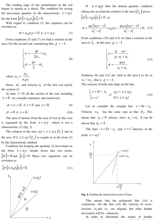
Let us consider the straight line
x
=
kt
−
x
0.
Velocity
υ
0 has the same sign as thatσ
0.
This means thatx
0>
0
always, sincea
2>
a
1.
It can beshown that
a
2<
k
.
The lines
x
=
kt
−
x
0 andt
=
t
*intersect at the pointx
=
a
1t
*.
Fig. 4. Finding the intersection point of lines.
This means that the polygonal line (14) is continuous. On the line (14) the velocity of cross-sections
υ
1andυ
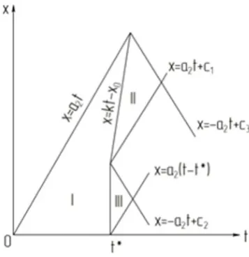
2 are aligned, but what further movement will be - unknown.problems for the first and second rods in the areas formed by the corresponding characteristics (fig. 5).
Fig. 5a. The geometric interpretation characteristics.
Fig. 5b. The geometric interpretation characteristics.
For the first rod in the area II the solution of the system (1) is sought in the form (3). Conditions are fulfilled at the border of the area II
x
=
kt
−
x
0:
(
)
(
2 0)
;
2 1 2 2 2 1
x
t
k
a
a
a
a
q
−
+
−
=
ρ
υ
(
)
(
2 0)
.
2 1 2 2 2 1
x
t
k
a
a
a
a
q
−
+
−
−
=
σ
(15)
In the area III for system (1) the solution is sought in the form (3). The following conditions are fulfilled at the border of the area III
0
≤
x
≤
a
1t
,
t
=
t
*(
)
;
2
2
2 1 1 2 2 2 2 0 *a
a
a
a
+
+
≡
=
ρ
ρ
ρ
υ
υ
υ
.
2 1 1a
a
x
a
q
+
−
=
σ
(16)
Also solving by the method of characteristics, we find a solution in the area III:
( )
* *;
2 1
1 1
1
ρ
χ
υ
υ
−
+
+
+
=
t
t
a
a
a
q
III.
2 1 1 1a
a
x
a
q
III+
−
=
σ
(17)
For the second rod in the area II the solution of the system (2) in the form of (4) is sought. The following conditions are fulfilled at the border of the area II
(
x
=
kt
−
x
0)
:
;
2
ρ
2υ
0υ
=
−
qt
+
.
2
2
0 0
+
−
=
qkt
σ
qx
σ
(18)
When solving this problem by the method of characteristics in the area II, we get:
(
) (
)
(
)
;
2
1
0 2 2 2 2 2 02
ρ
ρ
υ
χ
υ
−
+
−
+
−
+
=
qt
k
a
x
kt
x
qk
II(
) (
)
.
2
1
0 2 2 2 0 2 2 2σ
χ
σ
−
−
−
+
−
+
−
=
qx
k
a
x
kt
x
qa
IIIn the area III solution for a system (2) is searched in the form (4). The following conditions are
fulfilled at the border of the area III
0
≤
x
≤
a
1t
,*
t
t
=
,
*υ
υ =
.
2
σ
0σ
=
qx
−
(19)
Also solving by the method of characteristics, we find a solution in the area III:
( )
,
2
1
2
* *2
2
ρ
υ
χ
υ
III=
+
q
t
−
t
+
.
2
02
σ
σ
III=
qx
−
( )
( )
,
2
* * 2 2 * * 2 1
2 1
1
ρ
υ
υ
ρ
υ
υ
−
+
<
=
−
+
+
=
t
t
q
t
t
a
a
a
q
or
(
)
.
2
22 1 1
2
ρ
ρ
q
a
a
a
−
<
+
Which is a contradiction. The contradiction arose due to the assumption that in the area III
χ
=
−
1
. Therefore
χ
≠
−
1
. This means that in the area III rods move as a unit, i.e., their velocities are the same. Now consider the solutions for both rods in the area II. Suppose that in the area IIχ
=
−
1
,
i.e.2
1
υ
υ
<
. If we apply the designations that were entered earlier, we get:.
0
x
kt
x
>
−
This inequality is true for all
x
andt
which lie on the plane to the left of the straight linex
=
kt
−
x
0(Fig. 6).
Fig. 6. Area solutions.
We conclude that in the area II
χ
≠
1
. Subsequently rods will move as a unit, with the proviso that
χ
<
1
.
Heterogeneity in solutions arises by the fact that it is necessary to separate stresses in the first and second rods. The final solution is:(
)
1(
)
10( )
;
1
1
E
f
at
x
E
ϕ
at
x
σ
x
σ
=
+
+
−
+
(
)
2(
)
20( )
;
2
2
E
f
at
x
E
ϕ
at
x
σ
x
σ
=
+
+
−
+
(
)
(
)
( )
( )
10 20
.
af at
x
a
at
x
d
x
d
x
t
dx
dx
υ
f
σ
σ
ρ
=
+
−
−
+
+
+
(21)
In the area II we solve the system (21), provided that on its boundary
x
=
kt
−
x
0 :(
)
2 1 2 2
2 2 1 10
a
a
x
t
a
qa
−
−
−
=
σ
;
0 20
2
−
σ
=
σ
qx
;
.
2
ρ
2+
υ
0−
=
υ
qt
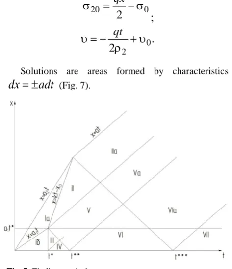
Solutions are areas formed by characteristics
adt
dx
=
±
(Fig. 7).Fig. 7. Finding a solution.
3 Results and discussion
The proposed method found solutions within each of the eleven areas, which are constructed using the method of characteristics. A full range of solutions has been obtained throughout the quadrant
Qualitative conclusions from the obtained solution of the problem can be obtained by considering the
dependence and at fixed (Figs.
8, 9a, 9b).
Fig. 8. Dependence of velocity on time.
Up to the moment
t
=
t
* velocityυ
1increases from zero to a certain valueυ
*and the velocityυ
2 decreases from a certain value to the same valueυ
*. Then the velocity of joint movement of rods increases according to linear law. At time,t
=
t
*** the rate is,
0
≥
x
t
≥
0
.
(
t
,
x
=
0
)
constant 2 2 0
.
ρ
υ
ρ
a
a
The fixed time
t
such thatt
<
t
*, the stress in the first rod in the area0
≤
x
<
a
1t
decreases by linear law from zero to a certain value, then at
a
1t
≤
x
≤
a
2t
, the valueσ
1 increases by linear law to zero. Whenx
>
a
2t
, the valueσ
1 remains zero. In the second rod, the stress increases from a value0
σ
−
to a certain valueσ
2 atx
=
a
2t
, ifx
>
a
2t
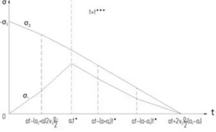
, the value is zero.Fig. 9a. Dependence of the stresses on the coordinate.
When
x
=
a
2t
leap occurs in the stress value for the second rod, since the edgex
=
a
2t
for it is a shock.Fig. 9b. Dependence of the stresses on the time.
At a fixed point in time
t
, such thatt
>
t
***, the stress in the first rod decrease linearly from zero to a certain valueσ
1 atx
=
a
1t
*.
Whenx
>
a
1t
* value1
σ
increases to zero by linear law and(
2 1)
2 0
2
a
a
q
at
x
>
+
υ
ρ
−
, the stress value remainsequal to zero in the first rod. Stress in the second rod increases by linear law from a value of
−
σ
0 to zero at(
2 1)
2 0
2
a
a
q
at
x
=
+
υ
ρ
−
and it remains equal tozero at
2
0 2(
a
2a
1)
q
at
x
>
+
υ
ρ
−
.4 Conclusion
The obtained analytical solution makes possible obtaining relations for stresses and strain rates in composite rods and materials. The results can be generalized to large number of layers with different properties and geometry. Such generalization will allow developing new mathematical models that are directly relevant to real technical products [11-13].
This work was carried out using equipment provided by the Center of Collective Use of MSUT "STANKIN".
References
1. E.N. Sosenushkin, Vestnik MSTU "STANKIN" 1, (2010) [in Russian]
2. A.G. Kobelev, Technology layered metal
(Metallurgy, 1991)
3. V.V. Emelyanov, Specification and rolling regimes bimetallic sheets for the manufacture of these products way rotary drawing (Blank production in mechanical engineering. №7. 2015)
4. C.B. von der Ohe, R. Johnsen, N. Espallargas
Multi-degradation behavior of austenitic and super duplex stainless steel - The effect of 4-point static and cyclic bending applied to a simulated seawater tribocorrosion system (Wear. Vol. 288, 2012)
5. A. Zmitrowicz Models of kinematic dependent anisotropic and heterogeneous friction.
(Int.J.Solids Struct, Vol. 43, 2005.)
6. L.V. Nikitin, Longitudinal vibrations of elastic rods in the presence of dry friction (Izvestiya AN SSSR, MTT. №6, 1978)
7. L.V. Nikitin, Wave propagation in elastic bar in the presence of dry friction (Engineering magazine, MTT, V.3. Vol. 1, 1963)
8. L.V. Nikitin, Rigid body shot by elastic rods with an external dry friction (Engineering magazine, MTT, №25, 1967)
9. L. Nikitin, A. Khamraev, E. Yanovskaya, Physics of the Earth and Planetary Interiors, 50, 26-31 (1988)
10. E.A. Yanovska, On the problem of the vibrations of the diaphragm, a lumped (Sat. "Numerical modeling in mechanical problems", Publishing house of the Moscow University, 1991)
11. V. I. Kolesnikov, A. L Ozyabkin, E.S. Novikov An innovative approach to the study of friction, wear, and monitoring of heavily loaded tribosystems (Friction and Wear., T. 40., No. 4, 2019)
12. V. M. Musalimov, K. A. Nuzhdin Modeling the external dynamics of frictional interaction using the theory of stability of elastic systems (Friction and Wear., T. 40., No. 1., 2019)
14. S.N. Grigoriev, M.P. Kozochkin, F.S. Sabirov, and A.A. Kutin, Diagnostic systems as basis for technological improvement, Proc. CIRP, 1, 599-604 (2012)
15. S.N. Grigoriev, V.A. Sinopalnikov, M.V. Tereshin, and V.D. Gurin, Control of parameters of the cutting process on the basis of diagnostics of the machine tool and workpiece, Measur. Techn., 55(5), 555-558 (2012)