MAINTENANCE OF GENETIC VARIABILITY UNDER THE PRESSURE OF NEUTRAL AND DELETERIOUS MUTATIONS IN A FINITE POPULATION

MAINTENANCE O F GENETIC VARIABILITY UNDER T H E PRESSURE O F NEUTRAL AND DELETERIOUS MUTATIONS

IN A FINITE POPULATION

WEN-HSIUNG L I

Center for Demographic and Population Genetics, University of Texas Health Science Center at Houston, Houston, Texas

Manuscript received July 5, 1978 Revised copy received November 3, 1978

ABSTRACT

In order to assess the effect of deleterious mutations on various measures of genic variation, approximate formulas have been developed for the frequency spectrum, the mean number of alleles in a sample, and the mean homozy- gosity; i n some particular cases, exact formulas have been obtained. The as- sumptions made are that two classes of mutations exist, neutral and deleterious, and that selection is strong enough to keep deleterious alleles in low frequen- cies, the mode of selection being either genic or recessive. The main findings are: (1) If the expected value ( G ) of the sum of the frequencies of deleterious alleles is about 10% or less, then the presence of deleterious alleles causes only a minor reduction in the mean number of neutral alleles ir, a sample, as compared to the case of G = 0. Also, the low- and intermediate-frequency parts of the frequency spectrum of neutral alleles are little affected by the presence of deleterious alleles, though the high-frequency part may be changed drasti- cally. ( 2 ) The contribution of deleterious mutations to the expected total num- ber of alleles in a sample can be quite large even if

4

is only 1 or 2%. (3) The mean homozygosity is roughly equal to (1-2G)/(1+81), where 8 , is twice the number of new neutral mutations occurring i n each generation in the total population. Thus, deleterious mutations increase the mean heterozygosity by about 2rj/ (1 +e,). The present results have been applied to study the contro- versial problem of how deleterious mutations may affect the testing of the neutral mutation hypothesis.

U S I N G WRIGHT’S ( 1949a) multiallelic distribution, I have recently developed formulas for the frequency spectrum, the mean number of alleles in a sam- ple, and the mean and variance of homozygosity under mutation pressure, under either genic or recessive selection (LI 1977, 1978; see also WATTERSON 1978a). These formulas are general, but become computationally intractable when the intensity of selection is strong. Simpler formulas are therefore needed for the case of strong selection. In some particular cases, I have recently been able to reduce my formulas to simple forms by algebraic manipulations, but I have not been able to do so in general. I have, however, used a heuristic approach similar to that of WRIGHT (1966) to get approximate formulas that are useful for the study of strong selection. Recently, W. J. EWENS (personal communication) has

pursued the same problem and has, somewhat earlier than I, obtained approxi- mate formulas for the mean number of alleles i n a sample and the mean homo- zygosity for the case of genic selection, using a different heuristic approach. M y results for this case largely agree with his. The purpose of this communication is to present my new results mentioned above and to apply them to investigate the controversial problem of how deleterious mutations may affect the testing of the neutral mutation hypothesis (EWENS 1972; NEI 1975; OHTA 1976; WAT- TERSON 1978b,c).

I n this study, I assume that there are two classes of mutations, neutral and deleterious, and that selection is sufficiently strong to keep deleterious alleles in low frequencies. Under certain circumstances, my approximate formulas for the frequency spectrum of neutral alleles are not very satisfactory. Nevertheless, they provide deep insight into the problem and enable us to compute fairly accurately both the mean number of neutral alleles in a sample and the mean homozygosity.

GENIC SELECTION

Consider a randomly mating population of effective size N . Let the number of possible allelic states at a locus be K, and let

Ai

denote the ith allele and x z its frequency. W e assume that there are two classes of alleles, i.e., neutral alleles and deleterious alleles, and that the neutral class consists of the first I allelic states and the deleterious class the remaining K - I states. Let s be the selection coeffi- cient against deleterious alleles. We use the K-allele model: each gene, of what- ever allelic type, ha5 a mutation rate U per generation and the probability of Ai mutating to Aj is u1 =

v/(K

- 1) for each j #

i, i

= 1,

. . .

,

K

(WRIGHT 1949b; KIMURA 1968a). Let p = x1

+

.

.

.

+

XI be the sum of the frequencies of neutral alleles and u1 = I u1 the sum of the mutation rates to neutral alleles; similarly, let q = xr+l

+

.

. .

+

xK and uz =

( K

- Z)u1. I n addition, let A = 4Nul,

el

= 4Nu1 = ICU, 8, = 4Nu, = ( K

-

I)cu, and OT = 4Nv =

O1

+

8,

-

A. In this paper,

we assume that s is at least one order larger than uz and that S = 4Ns is suffi- ciently large so that the expected value

( q )

of q at equilibrium is close to the equilibrium value in a population of infinite size, i.e.,

4

W e first study the frequency spectrum, which is conventionally denoted by

@(x)

and has the meaning that

@(x)dz

represents the mean number of alleles whose frequency is between z and x

+

dx.

(The frequency spectrum is also com- monly known as the distribution of allele frequencies.)

a ( ~ )

can be decomposed into the frequency spectrum of neutral alleles, (x), and the frequency spec- trum of deleterious alleles, a z ( x ) . We treat

@.,(XI

and @,(z) separately.

First, let us consider a2 (z)

.

To this end, we focus our attention on a particular deleterious allele, say A , ,

i

>

I . I t can be easily shown that the mean change of x, per generation is approximately given by

4

= u2/s =

e,/s.

Ma=7A(1-xz) - u z , - s z , p

.

GENETIC VARIABILITY 649

M y earlier computations for the case of I = 1 suggest that this approximation introduces no serious errors as long as S = 4Ns is larger than 20 (see Tables 1

and 4 of LI 1978). Putting the variance of the change in xi per generation equal to xi (1 - x i ) / ( 2 N ) , we find that the equilibrium probability density of xi is given by

in which

r(.)

is the gamma function. Since there are K

-

Z allelic states in the second class,

@z(x) = ( K - - l ) + ( x )

-

Letting K approach infinity, but keeping U and I / K constant, we obtain the fol- lowing result for the infinite-allele model:

cp,(x) =

e z x y i

- x ) s + w

.

(3)

(Note that, in the infinite-allele model,

el

+

O2 becomes equal to

e,.)

The ex- pected number of deleterious alleles in a random sample of m individuals or 2m genes is equal to

1

&

J

0 [ l - ( 1 - x ) 2 n ’ ] @ 2 ( ~ ) d x (4)

= e,[(S+

el)-1

+

(s+e,

+

q - 1

+

. . .

+

(s+e1+2m-

11-11

=

e2

iog,[(s

+

e,

+

2m

-

0.5)/(s+

e,

- 0.511

=

o2

loge[ 1

+

2 m / ( S

+

e, -

0.5)

1

.

_{( 5 )}

Using a different approach,

EWENS

(personal communication) has o,btained a slightly different formula:

(6)

=

8, loge [ 1

+

2m/ ( S

+

0 - 0.5) ]

.

The contribution to mean homozygosity due to deleterious genes is given by

which is negligibly small, if S is large. EWENS (personal communication) neg- lects this term by arguing that it is of order SF. The sample mean is expected to be slightly larger than the population mean given by ( 7 ) , but the difference is negligible as long as m is larger than 25 (cf., NEI and ROYCHOUDHURY 1974).

The same comment applies to formulas (14a,b).

W e now consider

a,

(5). The mean change of xi per generation for a neutral

allele

( i

5 I ) is approximately given by

Replacing q by u 2 / s , we find

From (9)

,

we obtain

al

(1)

=

e,+(i - s)el-l (10)

for the model of infinite alleles. This is identical with the frequency spectrum for the case of neutral mutations with effective size

N

and mutation rate u1 (KIMURA and CROW 1964). Thus, substituting for q in equation ; (8) i s

equivalent to neglecting the class of deleterious mutations. As will be seen later, this approximation creates no serious errors when 8, 2 1. However, serious dis- agreements between (IO) and the exact frequency spectrum occur at high allele frequencies when O1

<

1. Fortunately. even in this case, @,(I) in (IO) agrees extremely well with the exact frequency spectrum at low and intermediate allele frequencies, and gives a quite accurate value for the mean number of neutral alleles in the population. Consequently,

1

E,

=

j

[I - ( 1 -s)’”]@,(s)dz ₍₁₁₎

0

el

N - - 1 9 1 + L + . . . +

I91 8 , + 1 8 , + 2 m - I

provides, in all cases, a close approximation to the mean number of neutral alleles in a sample (see examples and a more detailed expanation below). EWENS (per- sonal communication) has obtained the same formula as (12a). This formula is expected to give a n Overestimate because it is obtained under the assumption that there exists no deleterious allele in the population.

Another estimate of

El

can be obtsined as follows. We again neglect the class of deleterious mutations, but assume that the effective population size is Njj

AT( 1 - u 2 / s ) instead of N . From these two assumptions, we get

in which 8,’ = 8, ( 1 - u 2 / s ) . This is a n underestimate because the actual effect of

random drift on neutral genes is weaker than that created by an effective size of When using @1 ( 5 ) in (IO) to compute

J1,

the contribution to mean homozy- gosity due to neutral genes, we must remember that this formula was obtained by assuming that the population is free of deleterious mutations and therefore every gene drawn from “the population” is neutral, i.e.,

j

x@,

(s)dz = I. Since N ( 1 - u2/s).

1

GENETIC VARIABILITY 65 1

instead of 1,

the actual probability of a randomly drawn gene being neutral is we need to multiply

1 1

P, = j- 22a,(s)ds = -L-

O 1

+ e ,

by j j z (1 - u2/s) in order to obtain

J1,

namely, - (I-uu,/s)2

J ,

=

i + e ,

.

This formula is identical with that of EWENS (personal communication). We

may roughly regard P, as the conditional probability that two genes randomly chosen from the population are of the same allelic type, given that they are neutral genes. As will be seen below, the actual frequency spectrum of neutral alleles is somewhat less dispersed over the whole allele frequency range than the approximate one given by (IO) ; consequently, P , is an underestimate. Because of this, formula (14a) tends to be a n underestimate; however, it may become a n overestimate when 8, is small and selection is weak, so that neutral alleles may temporarily become absent from the population and jj

<

1 - u2/s (see examples below). An overestimate for P , can be obtained by neglecting the class of deleterious mutations and assuming that the effective population size is

IV(

1 - u B / s ) instead of N . It is given by P, = 1/[1

4-

(1 - u 2 / s )

e,],

from which we get

-

J1-

( 1 - ~ ~ / ~ ) ~ / [ 1 + ( 1 - ~ ~ / ~ ) 0 ~ ]

.

(14b) Since P , is a n overestimate, so is formula (14b).

Making use of these formulas, we can compute

@(x)

= %(x)

+

a2(x),

k

=

xl

4-

Kz,

and

7

=

Jl

4-

7,)

in which is the mean total number of alleles in a sample and

7

the mean homozygosity of the population.

Let us now examine the accuracy of the above formulas. This can be done by comparing these formulas with my earlier ones (LI 1977, 1978) for reasonably large 4Ns values. To a close approximation, my earlier results can be written as follows.

cZ-l=

{

S"r(n+81)/[n!r(n+eT)]

.

When 8, and 8, are integers, some simplification of these formulas can be made. Given below are three examples.

For 8, = 1 and 6 , = r, r a positive integer, r-1

2=0

@' (z) = 271

-

27' fTS(1-8) ,2 si ( 1

-

z) i/i!

,

a2

(z) = rz-lcSx

,

(21

1

( 2 2 )

( 2 3 )

J z = r / ~

.

(24)

S i ( l - z ) i

,

(25)

( 2 6 )

- 1

J1=,-rS-'+r(r+1)/(2Sz)

,

For

O1

= 2 and O2 = r,

?=I

i)

2 2 1

+-@(I-*) ~

2r

@ ' ( S ) = 2 x 1 ( 1 - x ) --

@, (1) = r z l ( 1 - z) cSX

-

r2 ( S - r ) -W"

,

S - r S - r U

i!

[2Sz

-

3 ( r

+

1)s

+

( r

+

1 ) ( r

+

2 ) ]

,

- 1 r

J ' = 3 -

3 ( S - r ) S '

7,

= r ( ~ - 2 ) / ~ 3

.

( 2 8 )

For

O1

= 3 and O2 = r,

+'(z) = 3 ~ 1 ( 1 - z ) 2 - 3 z - 1 [ ( r + 1 ) r - r ( r - 1 ) S + ( r - l ) ( r - 2 ) S 2 / 2 ] - '

x [ r ( r - I ) S z ( l -z) - ( r + I ) r x ( 2 - x )

+

c S ( 1 - z )

Y

( r -

i

+

1) ( r -

i)si

( 1

-

x)

i/i!]

,

( 2 9 )

r

[ ( r

+

I ) r

-

r ( r - 1)s

+

(I - 1 ) ( r - 2)S2/2]-'

-

1

J 1 z T - q

x [ ( r - i p 4 - 5 ( r + i ) S 3

+

4 ( r + 1) ( r + 2 ) S 2

-

( r + l ) ( r + 2 ) ( r + 3 ) 1

,

( 3 1 )

GENETIC VARIABILITY , 653

( 3 2 ) hold with a high degree of accuracy, though some approximations have been made to simplify them. The mathematical manipulations involved in the deriva- tion are tedious, but the principle is rather simple and can be illustrated by the simplification of C, for the simplest case: 8, = O2 = 1. Namely,

m

cl-'=

z

( - S ) " n ! / [ n ! ( n f l)!] n=0

m

= (+)-I

I:

(--S)"+l/(n+ l ) !

n=o

m

= (+)-I [- 1

+

z

(-S)"/n!]

n=O

= (1-@)/S

.

The same principle can be applied to derive formulas for any integral 8, and 02.

Furthermore, using such formulas and the method of numerical interpolations, an approximate frequency spectrum of neutral alleles can be obtained for arbi- trary (integral or nonintegral) 8, and 02; numerical computations show that the spectrum thus obtained is quite accurate when

2

2, though it is not very satis- factory when 8,

<

2. (An example will be given below to illustrate this method

1 5

10

5

0 0

EXACT

...

APPROX M A T E

0,=0.1, 0,=2.5

0.5

GENE FREQUENCY

of interpolation.) For ease of discussion, we shall call formulas (15) to (32) the “exact” formulas, though terms of order cS have been neglected in some of these formulas.

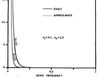
Figure 1 shows the approximate ( 3 ) and the exact frequency spectrum (16) of deleterious alleles for two cases: (1) S = 25, = 0.1, 0, = 2.5, and (2) S = 50,

0, = 0.1, 8, = 2.5. In both cases, the approximate frequency spectrum is almost indistinguishable from the exact one. Such close approximations also hold for larger Q l values. As an example, if O1 = 1 and O2 = r, formula (3) becomes

rz’(1 - z ) ” which is close to the exact frequency spectrum given by (22) as

long as S is large and r / S is small. As another example, if

O1

= 2 and 8, = r, formula ( 3 ) becomes r x l ( l -

x ) ~ + ~ ,

while the exact frequency spectrum is given by (26). The approximation is now even better. Thus, we may conclude that formula ( 3 ) holds well under the conditions specified in this paper. Numeri- cal computations suggest that formula ( 3 ) gives an underestimate, unless

el

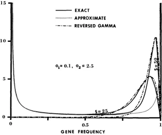
is large (cf., Figure 1).

The comparisons between the approximate (IO) and the exact frequency spectrum (15) of neutral alleles for the two cases given in Figure 1 are shown in Figure 2. Since the value is the same f o r both cases, so is the approximate

1 5

1 0

5

0

APPROXIMATE

.

. . .

. .

.

. . .

.-.-.-

REVERSED G A M M A

01= 0.1, O2

=

2.5

0 _0.5

GENE FREQUENCY

1

FIGURE 2.-Approximate and exact frequency spectra of neutral alleles for the same two cases shown i n Figure 1. The ordinate denotes +l(z), which has the meaning that +,(z)dz

represents the expected number of neutral alleles whose frequency is between z and z

+

dz.

Reversed gamma distribution. For detail, see text.

GENETIC VARIABILITY 655 frequency spectrum (10) because it is determined by 8, alone (see the dotted line), I t is seen from this figure that the approximate frequency spectrum agrees well with the exact one at low and intermediate allele frequencies, but deviates far from it at high allele frequencies. Such serious discrepancies are expected to arise whenever 8, is smaller than unity. The explanation is as follows: When 8, = 0 (in the absence of deleterious mutations),

@,(x)

is exactly given by (10) and is U-shaped, i.e., @, (x) has a peak at z = 1. As 8, increases, the probability of monomorphism decreases and the aforementioned peak becomes lower and moves inward; when 8,

+

8, = OT, becomes larger than one, @,(z) becomes zero at z = 1, and the peak moves to somewhere below

x

= 1 (see LI 1978). Since the approximate frequency spectrum (10) does not change with

e,,

the approxi- mation will become less and less satisfactory as 8, increases. Fortunately, the mean number of high-frequency alleles i n the population computed by using (1 0) is only slightly larger than that computed by using (15). For example, the mean number of alleles whose frequency is higher than 0.6 is 0.923 for the curve with S = 25, 0.942 for the curve with S = 50 and 0.959 for the approximate fre- quency spectrum given in Figure 2. Since the mean number of high-frequency alleles in a sample of reasonable size should be roughly the same as that i n the population, the discrepancies between the approximate and exact frequency spectra at high allele frequencies should introduce no serious errors into formula (12a), the approximate formula f o r the mean number of neutral alleles in a sample. That this is indeed the case can be illustrated by the following example: For the parameters specified in Figure 2 and 2m = 200, formula (12a) gives

k,

= 1.57 and formula (17) gives

g,

= 1.56 for the case of S = 2 5 , and 1.57 for the case of S = 50. More examples are given in Table 1.

15

1 0

5

0

...

APPROXIMATE

.-.-.-

BY INTERPOLATION

0 0.

s

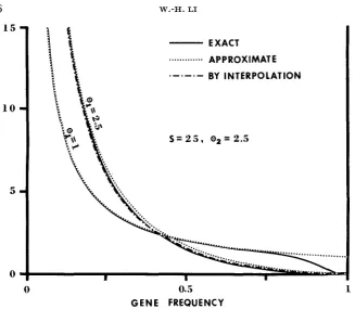
1

FIGURE 3.-Approximate and exact frequency spectra of neutral alleles for two cases of genic selection: ( 1 )

E , =

1, 8 , = 2.5, S = 25 and

(e)

8 , = 2.5, 8 , = 2.5, S = 25. The ordinate denotes a1(z), which has the meaning that @,(z)dz represents the expected number of neutral alleles whose frequency is between z and z f dz. - Exact frequency spectrum.

. . .

.

. .

Approximate frequency spectrum computed by using formula (IO).

-. -. -.

Extrapola- tion by using formulas (25) and (29).

GENE FREQUENCY

First, we note from Figure 2 that this part of a,

(x)

resembles a reversed gamma distribution. The following is the theoretical basis for this resemblence. When

O,/S

and 8, are small, the distribution of q, the sum of the frequencies of dele- terious alleles, can be approximated by the gamma distribution + ( q ) = G ( q ;

Y,, S ) in which

(NEI 1968). Since p , the sum of the frequencies o€ neutral alleles, is equal to

1 - q, the distribution of p can be approximated by the reversed gamma distribu- tion + ( p ) = G ( l

-

p ;

e,,

S ) . When 8, is very small, so that most of the time there is only one neutral allele in the population, a1(x) should follow + ( p )

closely except at frequencies near x = 0, where

a1(s)

is very large. When 8, becomes larger but is still substantially smaller than one, the high-frequency part of @,(x) should still resemble some reversed gamma distribution, though it will now have a lower peak and a longer tail, that is, the a and

p

values for

GENETIC VARIABILITY 65 7 Figure 2, the high-frequency part of the curve with S = 25 follows roughly the reversed gamma distribution with a: = 2 and

p

= 15, while that of the curve with S = 50 follows roughly the reversed gamma distribution with a = 1.9 and

p

= 27; these two distributions were obtained by trying some reasonable combinations of a: and

p

values. Second, we note further that the peak of + ( q ) should occur near

x

=

(e,

- 1)/S because the peak of G(y;a,P) is at y = (,a:

-

1)//3. There- fore, the peak of

a1

(z) should occur near

x

= 1 -

(ez

- l)/S. For example, the peak of the curve with S = 25 OCCLXS at x = 0.93, which is only slightly smaller than 1 - (0, - 1)/S = 0.94, and lhat of the curve with S = 50 occurs at z = 0.965, which is again only slightly smaller than 1

-

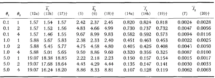
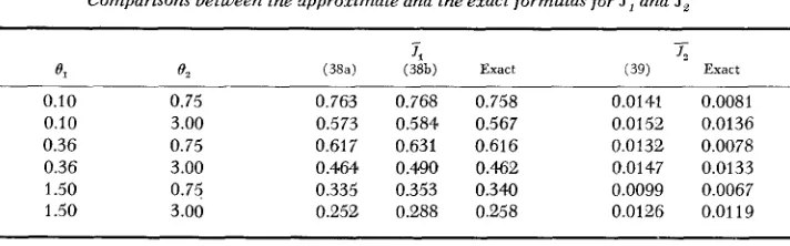
( 0 , - 1)/S = 0.970.

In Table 1, we examine the accuracy of the approximate formulas for X I ,

E?,

TI,

and

7,;

the "exact" formulas for these quantities are given by (1 7), (1 8)

,

(1 9) and (20), respectively. The parameters are specified in the table. We observe the following. (i) The accuracy of formula (12a) declines with increasing B,/S,

but remains quite high as long as e,/S is not considerably larger than 0.1; if

el

is around one o r smaller, formula (12a) is still fairly accurate even if 0,/S is 0.2. This result indicates that if the sum of their frequencies is 0.1 or smaller, the presence of deleterious alleles causes no substantial reduction in the mean num- ber of neutral alleles in a sample. Note that formula (12a) always gives a n over- estimate. Formula (12b) is less accurate than (12a), but provides a lower bound for the mean number of neutral alleles in a sample. (ii) Formula (5) is a close approximation to formula (18), and is somewhat better than formula (6), par- ticularly when 0, is large. I n most cases, formula

( 5 )

gives a n underestimate- it. becomes a n overestimate only when

el

is very large. (iii) Formula ( 1 4 4 gives a close approximation to formula (19) and is, on the whole, slightly better than iormula (14b). Note that the latter always gives a n overestimate while the former gives a n underestimate except for the case of

el

= 0.1 and 8, = 1. It has been explained earlier why formula (14a) may become an overestimate when selection is weak and O1 is small. Interestingly, if S and

e,

are raised to

_-

50 and 2.5,

TABLE 1

Comparisons between Ihe approximate and the exact fwmulas f o r k , ,

kz,

SI

and

Ts*

0.1 1 1.57 1.54 1.57 2.4a 2.37 2.45 0.820 0.824 0.818 0.1 2 1.57 1.52 1.56 4.83 4.66 4.99 0.730 0.737 0.732 0.1 4* 1.57 1.46 1.55 9.687 8.99 9.83 0.582 0.592 0.573 1.0 1 5.88 5.67 5.83 2.38 2.33 2.40 0.451 0.463 0.453 1.0 2 5.88 5.4'5 5.77 4.75 4.58 4.80 0.4805 0.426 0.408 1.0 4 5.88 5.01 5.65 9.50 8.86 9.60 0.320 0.356 0.325 5.0 1 19.07 18.38 18.85 2.22 2.18 2.23 0.150 0.157 0.154 5.0 2 19.07 17.68 18.64q 4.43 4.29 4.44 0.135 0.147 0.141 5.0 4 19.07 16.24 18.20 8.86 8.33 8.81 0.107 0.128 0.119

0.0024 0.0028 0.0047 0.0056 0.0094 0.01 16 0.0022 0.0025 0.004.; 0.0050 0.0087 0.0100 0.0015 0.0017 0.0030 0.0033 0.0062 0.0063

* S = 20,2m = 200. The numbers in parentheses refer to formula numbers.

but 0, remains equal to 0.1, then formulas (14a) and (19) both give

1,

= 0.820; note that the value of e,/S is the sallie as that of 1/20. (Because of computational difficulty, no larger S has been tried.) This suggests that if

S

is large, formula

(14a) will become an underestimate even if

el

is small and the exact value of will be somewhere between the two values given by (14a) and (14b), probably closer to the former. (iv) Formula ( 7 ) is a close approximation to formula (20) a n d J 2 is usually negligible. Note that the 3 value used in Table 1 is only 20. When S is larger, the agreement between the approximate and the “exact” formulas is expected to be even better. This has been borne out by extensive computations.

RECESSIVE SELECTION

Let the fitness of A,A, be 1 - 2s if

i.

i

>

1 and one if otherwise. This means that the deleterious alleles are completely recessive. W e use the same notations as above and make the same assumption that Q is close to Q =\l‘u2/(2s) = d/e,/(2S), the equilibrium value in an infinite population.

W e again focus our attention on the frequency of a particular deleterious allele, say Ai,

i

>

1. It can be easily shown that the mean change of zz per gen- eration is given by

Mi = v , ( l - z % ) - uxt - 2sx,(l - q ) q

,

M ,

=

V l ( l

-x,)

- x * ( d G + U1 - v,)

.

approximately. As WRIGHT (1 966) did, we replace q by

4

and find that (33)

A - comparison of (33) with (1) suggests that if we substitute \/2u2s for s (or d 2 8 , S for S ) in the approximate formulas for genic selection, we will obtain the corresponding formulas for recessive selection. This is indeed the case and we have the following:

-

-

k,

=

0, l o g e [ l + 2 m / ( q m + 8, - 0.5)]

,

GENETIC VARIABILITY 659

4

=

r[e,

4-

1)/2]/[V/Sr(e2/2)] should be used (NEI 1968). Numerical com- putations show that, as in the case of genic selection, formula (35) gives a close approximation to the frequency spectrum of deleterious alleles, and i n what fol- lows we shall be concerned only with the accuracy of formulas other than (35) and (37). The corresponding “exact” formulas have been given by LI (1977, 1978).

Figure

4

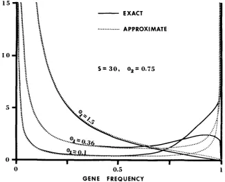
shows the approximate (34) and the exact frequency spectrum of neutral alleles for three cases: 8, = 0.1, 0.36, and 1.5; in all cases, S = 30 and Q 2 = 0.75. It is seen that in the first two cases the approximate frequency spec- trum agrees well with the exact one at low and intermediate allele frequencies but deviates far from it at high frequencies, while in the third case there occur no large discrepancies. As in the case of genic selection, the approximate and the exact frequency spectrum give similar values for the mean number of neutral alleles whose frequency is higher than 0.01; for the above three cases, the former gives 1.50,2.70, and 6.86, and the latter gives 1.47,2.44, and 6.73. Consequently, formula (36a) holds fairly well; for the same three cases as above, it gives 1.73, 3.52, and 10.31 if 2m = 1000, while the exact values are 1.72,3.49, and 10.18.

Table 2 shows some comparisons between the approximate and the exact

- -

S = 30, 0 2 = 0.75

15

LO

5

0 0.5 1

G E N E F R E Q U E N C Y

FIGURE 4.-Approximate and exact frequency spectra of neutral alleles for three cases of recessive selection: e, = 0.1, 0.36, 1.5; in all cases, e, = 0.75 and S = 30. The ordinate denotes

@,(z), which has the meaning that +p,(z)dz represents the expected number of neutral alleles

formulas for J , and

1,.

It is seen that formula (38a) gives a quite accurate value for

5.

The S value used is only 30 and formula (38a) tends to give a n over- estimate. If S becomes large, this formula will probably become a n underestimate; unfortunately this is difficult to verify, because of computational difficulties. Formula (38b) is less accurate than formula (38a), but provides an upper bound for

J,.

Formula (39) tends to give an overestimate for

T2,

particularly when 8 2 is small. Fortunately, when S becomes larger than 50,7, becomes less than 0.01 because it can be shown that

7,

<

1/(2S)

,

and can therefore be neglected.

E S T I M A T I N G 6 F O R T E S T I N G THE N E U T R A L M U T A T I O N H Y P O T H E S I S

It has been controversial as to how one should estimate 8 when testing the neutral mutation hypothesis. On the one hand, NEI

(NEI

and ROYCHOUDHURY

1974; NEI 1975), OHTA (1976) and some others advocate using the estimator given by

8 , = h / ( l - A )

,

(40)

in which h is the observed mean heterozygosity of the population f o r a large num- ber of loci. On the other hand, EWENS (1972) and

WATTERSON

(1978b,c) con- tend that it is better to use the estimator defined through

7 (41 )

i k ik

+ . . . +

A = - + - i k

i k 6 k f 1 ik4-2m-1

in which k is the total number of alleles observed in a sample for a single locus. I n my opinion, this controversy arises because of the failure to distinguish be- tween the hypothesis of pan-neutrality (H,)

,

which postulates that all alleles in a population are neutral, and the hypothesis of neutral mutations ( H n ) , which postulates that the genic variation or the heterozygosity of a population is mainly due to neutral or almost neutral mutations. These two hypotheses may appear similar superficially, but are actually very different. In fact, H p is much more stringent than

H,.

The following example will make this point clear. Suppose

TABLE 2

Comparisons between the approximate and the exact formulas for

TI

and

Tg*

0, 0.10 0.10 0.36 0.36 1.50 1.50 0 2 0.75 3.00 0.75 3.00 0.75 3.00 ~~ (38a) 0.763 0.573 0.61 7 0.464 0.335 0.252 j*

(38b) Exact

0.768 0.758 0.584 0.567 0.631 0.616 0.440 0.462 0.353 0.340 0.288 0.258

-

'2

0.0142 0.0081 0.0152 0.0136 0.0132 0.0078 0.0147 0.0133 0.0099 0.0067 0.0126 0.01 19

(39) Exact

GENETIC VARIABILITY 661 that at a certain locus there are six alleles with the following frequencies: 0.60, 0.36, 0.01, 0.01, 0.01, 0.01. Then, for H , to hold, it requires only that the first two alleles be neutral because the heterozygosity is mainly due to these two alleles. But, for H , to hold, it requires that all six alleles be neutral; if any one of them is not neutral (say, one of the four low-frequency alleles is deleterious), then H , is not true, In other words, H , can be true even if the majority of the alleles are deleterious, but H , is true only if every allele is neutral. This differ- ence is of vital importance because the majority of mutations are deleterious and every natural population contains many deleterious genes. W e note that what KIMURA (1968a,b) proposed is not H , but H,. I n NEI’S and OHTA’S approaches to testing H,, one needs first to estimate 8. The 0 value to be estimated is not OF,

the total 4 N u value, but

el,

the “neutral only” value, because H , postulates that only neutral mutations are important to the polymorphism of a population. HOW-

ever, since H , does not specify precisely what proportion of the mean hetero- zygosity is due to (almost) neutral mutations, only rough estimates of 0, can be obtained under this null hypothesis. In the method advocated by NEI (1975) and OHTA (1976), it is assumed that h is completely due to neutral mutations, ignoring the possibility that some (or many) of the rare alleles in the sample may be deleterious. This method has been criticized by EWENS (1972; personal communication) and WATTERSON (1978b,c), who argue that

&

is superior to because

k

is a sufficient statistic for

e

if all mutations (alleles) are neutral. This argument is valid if what is to be tested is H , or what is to be estimated is OT.

Here, however, the purpose of estimating 0 is to test H,, that is, what is to be estimated is

O1.

Since both estimating procedures ignore the possibility that some

of the rare alleles may be deleterious, we need to examine the effect of deleterious mutations on

&

and

&,

when comparing them as estimators of 0, under the null hypothsis of H,. I n the following, I shall use a numerical example to illustrate that the first approach is quite robust against the existence of rare deleterious alleles, whereas the second approach is not.

I

shall also discuss the controversial question of whether it is better to pool data €ram all loci studied or to treat each locus separately, the former approach being advocated by NEI (1975) and OHTA

( 1976) and the latter by W A T T E R ~ O N (1978b,c).

Effect of deleterious mutations: Assume that the genome consists of a large number of identical loci; the problem of inhomogeneity among loci will be dis- cussed later. Assume further that the parameter values for each locus are

el

= 1, 0, = 10, and S = 500, the mode of selection being genic. Using formulas (23)

and (24), we find that the mean heterozygosity of the population is

fl

= 0.52.

each locus is reasonably large (NEI and ROYCHOUDHURY 1974). Using h = 0.52

and equation (40)

,

we find t& = 1.08, which is reasonably close to 8, = 1. Next,

let us consider the second approach. This approach uses single-locus data but, for ease of comparison, let us neglect the sampling error and assume k =

x.

If

2m = 200, then

El

z 5.88,

k,

z 3.36 and

x

z 9.24. Using k 9.24 and equation

(41), we find f& 1.78, which is considerably larger than = 1. Thus,

&

is

quite sensitive to the existence of rare deleterious alleles, but O h is rather robust

against such alleles.

Now see what we will get if we use these two estimated values to make predic- tions. First, consider the mean heterozygosity. If we assume that 6' = 8h = 1.08

and all mutations are neutral, we will predict a heterozygosity of 1.08/ (1

4-

1.08) = 0.52. As expected, this is equal to the mean heterozygosity. On the other hand, if we assume that 8 =

&

= 1.78 and all mutations are neutral, we will predict a heterozygosity of 0.64, with a standard deviation equal to 0.16 (STEWART 1976). The difference between this predicted heterozygosity and the mean heterozygosity is 0.12, which is comparable to the standard deviation. This

result suggests that if the discrepancy between the observed mean heterozygosity among loci and the value predicted by using 8 = 8 k is used to test H,, there will

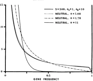
be a high probability of rejecting H , when H , is true, i.e., the type I error will be high. Next, consider the frequency spectrum. W e again assume that all muta- tions are neutral and 6' = 8 h for the first approach, while 8 = 8 k for the second approach. The frequency spectrum obtained by the first approach is represented by the curve with 8 = 1.08 in Figure 5, while that obtained by the second ap- proach is represented by the curve with 8 = 1.78. It is seen that the former is very close to the solid line, the actual frequency spectrum, but the latter deviates far from it. Again we see that the type I error is high for the second approach. It is interesting to note that in the present example 81c is much smaller than

BT =

11, and the spectrum with 8 = 1.78 is very different from that with 8 = 11. If our purpose is to test H,, we should try to get a more accurate estimate of 01- so that the spectrum obtained will be closer to that with 8 = 11. F o r this purpose, it is better to use NEI'S (1977) approach of estimating Q T through the number of rare

alleles than to use (41).

One might argue that in practice deleterious alleles may bz usually too rare

to appear in a sample, so that the second approach can also be applied to estimate

GENETIC VARIABILITY 663

15

1 0

5

0

0 0.5

G E N E F R E Q U E N C Y

1

FIGURE 5.-Frequency spectra under various situations. The ordinate denotes @ (x), which has the meaning that +(x)dx represents the expected number of alleles whose frequency is between x and x f dx. __ Genic selection with S = 500, 8 , = 1, e, = I O . .

. .

.

.

. Neutral mutations.

all these possibilities are taken into consideration,

k,

may easily become 1 or larger. Let us assume that this is true. Let us assume further that

I

0.2. Then, in a sample of 200 genes, the expected number of different neutral alleles is smaller than 2.12 and, on the average, about one third of the total number of alleles in the sample is due to the presence of deleterious mutants. The assump- tion of 8,

I

0.2 is quite reasonable because, if 8, = 0.2, the mean heterozygosity is greater than 0.16, which is roughly equal to o r larger than the majority of mean heterozygosities observed in Drosophila species (cf., AYALA et al. 1974 and data cited in NEI 1975). Although this assessment of the effects of deleterious mutations on

k

is admittedly rough and is based on data from Drosophila only, it suggests that the second approach of estimating 8 can be very unfavorable for the testing of

Hn.

Single-locus approach vs pooling data: A single-lccus approach generally has the following three drawbacks: ( i ) The estimator of a parameter often has a large mean square error. This is true for I& because

k

has a large variance (EWENS

thesis to be tested is H,, not to mention the less stringent hypothesis H,. As an example, let us consider

WATTERSON'S

(1978a,c) homozygosity test. This seems to be the best single-locus test that has been devised €or testing H p . Yet, his results show that it is almost impossible to reject H , if the sample contains fewer than three alleles (see Table 1 of

WATTERSON

1978a). (iii) Far testing H,, we will not be able to use data from monomorphic loci, loci with low heterozygosity, because such loci contribute little to the observed average heterozygosity and therefore whether the alleles at such a locus are neutral or not is an irrelevant question under the null hypothesis of H,. We note that the proportion of monomorphic loci is high in most of the species surveyed ( c f . , FUERST, CHAKRABORTY and NEI

1977). Thus, a large amount of iniormation will be wasted if we use a single- locus test. These three drawbacks can be overcome by pooling data from all loci studied. Of course, pooling data creates the problem of inhomogeneity because mutation rate varies from locus to locus and the mode and intensity of selection may also vary. However, the variation in mutation rate among loci may be taken into account by using a model of varying mutation rate as developed by

NEI

and his associates (cf., NEI, CHAKRABORTY and

FUERST

1976; FUERST, CHAKRA- BORTY and NEI 1977), though the problem of variation in the mode and intensity of selection among loci cannot be easily handled. At any rate, if the inhomo- geneity among loci is not taken into consideration in a test, the type I error may become large.

In addition to the above, some other arguments have also been put forward by both sides.

I

discuss two of them here. Both are arguments against the first ap- proach, namely, that o h has a large mean square error and a large bias. These two criticisms can easily be refuted because they are based on single-locus esti- mation, but what NEI (1975) and OHTA (1976) propose is to estimate the average 6, value among loci by using data from a large number of loci. Obviously. if data from a large number of loci are used, the mean square error of will become very small. This is also true for the bias for estimating the average 8, over the loci studied because it can be shown that the bias decreases quite rapidly as the number of loci used increases. Incidentally, even for a single-locus estimate. the bias of

&

may be a less serious problem than the sensitivity of

6,'

to the effect of deleterious mutations. For instance, for the example given in Figure

5 ,

adding a bias of 40% to O h increases its mean value from 1.08 to 1.51, which is still con- siderably better than the estimate

&

= 1.78. A bias of 40% is used in the above computation because EWENS (personal communication) argues that the simula- tion result of EWENS and GILLESPIE (1974) shows that for O T of order one the bias of @IL f o r a single-locus estimate is consistently 40% or more upwards, as-

suming that all mutations are neutral.

Several further remarks are in order. First, in the above I have compared

GENETIC VARIABILITY 665 whose sample frequency is, say, higher than 0.01. This approach is, however, more complicated than that using h. I n a future study, I shall examine whether the estimate obtained by the latter approach is close to that obtained by the former. If the answer is yes, then the latter is to be preferred to the former since it is much simpler. Second, although I have used a single-locus example to illus- trate the difference between H , and

H p ,

it should be borne in mind that Hn is postulated as a majority rule f o r the loci of a genome, and whether it is true or not can be decided only by studying a large number of loci. Third, it may be possible to find a statistic for testing H , whose distribution is free of the nuisance parameter 8, but so far no such test statistics have been found. W e note that although the testing procedures of EWENS (1972) and WATTERSON (1978a,b) do not require the estimation of 8, they are developed under the null hypothesis

of H,, not H,. Fourth, since the neutral mutation hypothesis was proposed, terms such as the neutral alleles hypothesis (or theory), the neutrality hypothesis, etc., have appeared in the literature. These terms have been used sometimes as equivalents for the neutral mutation hypothesis and sometimes as equivalents for the hypothesis of pan-neutrality. This is very confusing. I suggest that a clear distinction always be made between the two hypotheses. Fifth, some authors (e.g., WATTERSON 1978a,c) seem to think that “detecting selection among alleles” is equivalent to “testing the neutral mutation hypothesis,” but it is not. T o test the neutral mutation hypothesis is to detect selection among polymorphic alleles only, i.e., among alleles whose frequencies are higher than 0.01, say. Detecting selection among alleles is equivalent to testing the hypothesis of pan-neutrality. Sixth, whether an allele is almost neutral or not is judged by whether random drift or selection plays a more important role in the population dynamics of this allele. KIMURA (1968a) proposed the definition 12Nsl

<

1 but I (LI 1978) sug- gested that a better definition would be 1Nsl

<

1.

DISCUSSION

In obtaining the present theoretical results, it has been assumed that all dele- terious mutations have the same selective disadvantage. This assumption may seem restrictive, but from the results we may draw the following general con- clusions for the effects of de€eterious mutations on the frequency spectrum, the

mean number of alleles in a sample and the mean homozygosity:

First, if the expected value

( 4 )

of the sum of the frequencies of deleterious alleles is around 10% or less, then the presence of such alleles causes no sub- stantial reduction in the mean number oE neutral alleles in a sample. Further- more. the low and intermediate allele frequency parts of the frequency spectrum of neutral alleles are little affected by the presence of deleterious allels, though the high allele frequency part may be changed drastically.

Second, it can be shown that if S is much larger than 2m, then formula (5),

The same __ is true for formula (37), the formula for recessive selection, provided that d2B2S is much larger than

em.

Thus, a general principle emerges, namely, that the mean number of severeZy deleterious alleles in a sample is equal to the product of the sample size (2m) and the sum of the expected frequencies of such alleles (Q)

.

(Here, by severely deleterious alleles, we mean alleles with large S.)

W e note that if 2m = 200 and Q = 0.01, then formula (42) gives

&

2, a large value. Thus, the contribution of deleterious mutations to

%

can be quite large even if Q is only 1 or 2

% .

Third, the presence of deleterious alleles reduces the mean homozygosity of a

population from 1/( 1

+

0,) to about

Thus, the contribution of deleterious mutations to the meaii heterozygosity of a population is roughly equal to 2g /( 1 f

e,).

An upper bound of the mean homo- zygosity is given by

Of course, the second and third principles do not apply to the case where one or more of the deleterious alleles enjoy heterozygote advantage. These three principles are mainly for assessing the effects of mutations whose selective dis- advantage is considerably large. The effects of mutations with very mild dele- terious effect. say S

I

30, can be studied by my earlier formulas

(LI

1977. 1978).

I am indebted to W. J. EWENS for showing me his unpublished results and valuable com- ments. I also thank M. NEI, J. F. CROW and M. J. SIMMONS for discussions and suggestions. This study is supported by National Science Foundation grant DEB 77-09120 and Public Health Service grants GM 20293 and GM 19513.

LITERATURE CITED

AYALA, F. J., M. L. TRACEY, L. G. BARR, J. F. MCDONALD, and S. PEREZ-SALAS, 1974 Genetic variation in natural populations of five Drosophila species and the hypothesis of selective neutrality of protein polymorphisms. Genetics 77: 343-384.

The sampling theory of selectively neutral alleles. Theoret. Pop. Biol. 3:

87-112.

Some simulation results for the neutral allele model, with interpretations. Theoret. Pap. Biol. 6: 35-57.

Statistical studies o n protein polymorphism in natural populations. I. Distribution of single locus heterozygosity. Genetics 86 : 455-483.

Genetic variability maintained in a finite population due to mutational production of neutral and nearly neutral isoalleles. Genet. Res. 11: 247-269. -, 19681,

The number of alleles that can be maintained in a finite population. Genetics 49 : 725-738.

EWENS, W. J., 1972

EWENS, W. J. and J. H. GILLESPIE, 1974

FUERST, P. A., R. CHAKR~BORTY and M. NEI, 1977 KIMURA, M., 1968a

GENETIC VARIABILITY 667

Maintenance of genetic variability under mutation and selection pressures in

, 1978 Maintenance a finite population. Proc. Natl. Acad. Sci. U.S. 74: 2509-2513. -

of genetic variability under the joint effect of mutation, selection, and random drift. Genetics 90: 349-382.

The frequency distribution of lethal chromosomes in finite populations. h o c . Natl. Acad. Sci. U.S. 60: 517-524. -, 1975 Molecular Population Genetics and Evolution. North-Holland, Amsterdam. __ , 1977 Estimation of mutation rate from rare protein variants. Am. J. Human Genet. 29: 225-232.

NEI, M., R. CHARRABORTY and P. A. FUERST, 1976 Infinite allele model with varying mutation rate. Proc. Natl. Acad. Sci. U.S. 73: 4164-4168.

NEI, M. and A. K. ROYCHOUDHURY, 1974 Sampling variances of heterozygosity and genetic distances. Genetics 76: 379-390.

OHTA, T., 1976 Role of very slightly deleterious mutations in molecular evolution and poly- morphism. Theoret. Pop. Biol. 10: 254-275.

SIMMONS, M. J. and J. F. CROW, 1977 Mutations affecting fitness in Drosophila populations. Ann Rev. Genet. 11: 49-78.

STEWART, F. M., 1976 Variability in the amount of heterozygosity maintained by neutral mutations. Theoret. Pop. Biol. 9: 188-201.

WATTERSON, G. A., 1978a -,

19781, An analysis of multi-allelic data. Genetics 88: 171-179. -, 1978c The neu- tral alleles model, and some alternatives. Int. Stat. Inst. Conf. Proc., in press.

Adaptation and selection. pp, 365389. In: Genetics, Paleontology and Evolution. Edited by G. L. JEPSON, G. G. SIMPSON and E. MAYR. Princeton Univ. Press, Princeton, New Jersey.

-

,

1949b Genetics of populations. Encyclopaedia Britannica, 14th ed. 10: 111-112. ---, 1966 Polyallelic random driIt in relation to evolution. Proc. Natl. Acad. Sci. U.S. 5 5 : 1074-1081.

Corresponding editor: B. S. WEIR

LI, W.-H., 1977

NEI, M., 1968

The homozygosity test of neutrality. Genetics 88: 405-417.