Side-Channel Analysis: Side-Channel Atomicity
[Cryptology ePrint Archive, Report 2003/237]
Benoˆıt Chevallier-Mames1, Mathieu Ciet2, and Marc Joye1
1 Gemplus S.A., Card Security Group
La Vigie, Av. du Jujubier, ZI ATh´elia IV, 13705 La Ciotat Cedex, France {benoit.chevallier-mames,marc.joye}@gemplus.com
http://www.gemplus.com/smart/ 2
UCL Crypto Group, Universit´e catholique de Louvain Place du Levant 3, 1348 Louvain-la-Neuve, Belgium
ciet@dice.ucl.ac.be −http://www.dice.ucl.ac.be/crypto/
Abstract. This paper introduces simple methods to convert a cryp-tographic algorithm into an algorithm protected against simple side-channel attacks. Contrary to previously known solutions, the proposed techniques are not at the expense of the execution time. Moreover, they are generic and apply to virtually any algorithm.
In particular, we present several novel exponentiation algorithms, namely a protected square-and-multiply algorithm, its right-to-left counterpart, and several protected sliding-window algorithms. We also illustrate our methodology applied to point multiplication on elliptic curves. All these algorithms share the common feature that the complexity is globally unchanged compared to the corresponding unprotected implementations.
Keywords. Cryptographic algorithms, side-channel analysis, protected im-plementations, atomicity, exponentiation, elliptic curves.
1
Introduction
According to Goldreich [1], cryptography deals with the conceptualization, def-inition and construction of computing systems that address security concerns. We would like to add that cryptography is also concerned with concrete imple-mentations of such systems. This in turn implies that not only the systems but alsotheir implementations must withstand any abuse or misuse.
Suppose that (part of) an algorithm consists of a loop where the execution of a given set of instructions depends on certain input values. If from some side-channel information (e.g. timing or power consumption) one can distinguish which set of instructions is processed, then one can retrieve some secret data (if any) involved during the course of the algorithm. This is the basic idea behind simple side-channel attacks.
For example, imagine that, at a given step, a secret bit is used to select processΠ0orΠ1. A straightforward counter-measure against simple side-channel
attacks consists in making processesΠ0andΠ1indistinguishable. This is usually
achieved by executing processΠ0followed by a fake execution of processΠ1when
processΠ0 must be executed, and by executing a fake execution of processΠ0
followed by process Π1 when process Π1 must be executed. Such a solution is
however unsatisfactory from a computational perspective because the running time can be increased by a non-negligible factor.
In a sense, our approach refines this obvious solution, as much as possible. By potentially inserting dummy (fake) operations, we divide each process so that it can be expressed as the repetition of instruction blocks which appear equivalent by side-channel analysis. Such a block is called aside-channel atomic block. Building on this, we develop several approaches for unrolling the whole
code so that it appears as anuninterrupted succession of the processes. In other words, the whole code appears as a succession of blocks that areindistinguishable
by simple side-channel analysis. Remarkably, contrary to previous solutions, the techniques we propose areinexpensive and present the additional advantage of being fullygeneric,i.e.they apply to a large variety of cryptographic algorithms. The rest of this paper is organized as follows. In the next section, we define the notion of side-channel atomicity. We explain how to efficiently convert a cryptographic algorithm into an algorithm protected against simple side-channel attacks. Then, in Sections 3 and 4, we provide concrete applications to the RSA cryptosystem and to elliptic curve cryptosystems. Finally, we conclude in Section 5.
2
Side-Channel Atomicity
2.1 Side-channel atomic blocks
We view a process as a sequence of instructions. We say that two instructions (or a sequence thereof) areside-channel equivalent if they are indistinguishable through side-channel analysis. This relation is denoted by symbol “∼”. From this, we define what we call acommon side-channel atomic block.
Definition 1 (Side-channel atomicity [5]). Given a set of processes {Π0,
. . . , Πn}, a common side-channel atomic block Γ for Π0, . . . , Πn is a
side-channel equivalent sequence of instructions so that each process Πj (0≤j≤n)
can be expressed as the repetition of this block Γ, i.e. there exist sequences
γj,i∼Γ s.t. Πj =γj,1kγj,2k · · · kγj,`j. The instruction sequences γj,i are called
A common side-channel atomic blockΓ always exists by noticing that fake instructions can be artificially added to an existing process to make the differ-ent processes indistinguishable. The main difficulty resides in finding a blockΓ which is small with respect to some metric (e.g.running time, code size, . . . ). We note that a possible rearranging and/or rewriting of the processes may shorten Γ or limit the number of dummy operations and thus improve the overall per-formances.
2.2 Illustration
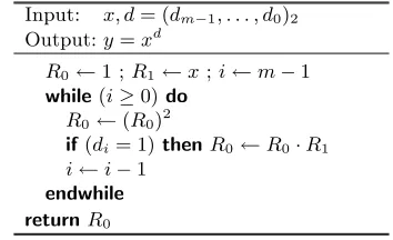
Before going further, we quote a simple example: the square-and-multiply algo-rithm. On input of an elementx in a (multiplicatively written) groupGand the
binary expansion of exponent d, d= (dm−1, . . . , d0)2, the square-and-multiply
algorithm returnsy=xd.
Input: x, d= (dm−1, . . . , d0)2 Output:y=xd
R0 ←1 ;R1←x;i←m−1 while(i≥0)do
R0←(R0)2
if(di= 1)thenR0←R0·R1 i←i−1
endwhile
returnR0
Fig. 1.(Unprotected) square-and-multiply algorithm.
As aforementioned, a valid choice for common side-channel atomic Γ con-sists of a squaring followed by a (possibly fake) multiplication and a counter decrementation. This algorithm is the well-known square-and-multiply always
algorithm [6]. This is the classical way for preventing simple side-channel at-tacks in the square-and-multiply algorithm.
Such a choice for Γ is suboptimal. Assuming that (i) a squaring operation can be performed by calling the (hardware) multiplication routine, and (ii) in-structionsR0←R0·R0 andR0←R0·R1 are side-channel equivalent,3 we can
rewrite the previous algorithm to clearly reveal a shorter common side-channel block Γ (see Fig. 2-a). Remark the fake instruction i ← i−0. Of course, we assume that this instruction is side-channel equivalent toi←i−1.
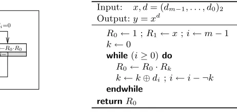
As depicted in Fig. 2-a, the algorithm is not balanced. There are two copies of Γ when di = 1 and only one when di = 0. However, as explained in the next section, it is easy to unroll the code so that a side-channel analysis only reveals a regular succession of copies of Γ without enabling to make the distinction
Decision di=0
di=1
R0←R0·R0 i←i−0
R0←R0·R1 i←i−1
Π0
Π1 R0←R0·R0 i←i−1
Γ =
Input: x, d= (dm−1, . . . , d0)2 Output:y=xd
R0←1 ;R1←x;i←m−1 k←0
while(i≥0)do R0←R0·Rk
k←k⊕di ;i←i− ¬k endwhile
returnR0
(a) Synopsis. (b) Side-channel atomic
square-and-multiply algorithm.
Fig. 2.Protected square-and-multiply algorithm.
amongst the processes being executed (i.e. Π0 or Π1). After simplification, we
obtain the algorithm presented in Fig. 2-b.
It is worth noting that our protected algorithm (Fig. 2-b) only requires 1.5m multiplications, on average, for computingy=xd, that is, the complexity of the usual, unprotected square-and-multiply algorithm (Fig. 1).4
2.3 General methodology
Given different processes Π0, . . . , Πn, we first identify a common side-channel atomic blockΓ. Next, we write the processes Πj (0≤j ≤n) as a repetition of Γ,i.e. Πj=γcjk · · · kγcj+`j−1 where`j is the number of copies ofΓ in Πj,
c0= 0
cj=cj−1+`j−1 for 1≤j≤n
and withγk∼Γ for allc0≤k≤cn+`n−1. Our strategy is to executeexactly `j times a sequence side-channel equivalent to Γ for process Πj. As a result, denoting byt the running time for Γ, the time required for processingΠj will only be`j·tinstead of (max0≤j≤n`j)·tfor the trivial solution.
In order to chain the different processes, we use a bit, says, to keep track when there are no more blocksγk ∼Γ to be executed when processingΠj. When processΠj is terminated (and thuss= 1), we have to execute the next process according to the input values of the algorithm. Moreover, at the beginning of each loop, we updatek, the number of the current sequenceγ, as
k←(¬s)·(k+ 1) +s·f(input values) 4
so that f(input values) =cj0 if the next process to be executed is Πj0. We see that whens= 0 then the value of k is incremented by 1. Of course, the above expression for k must be coded in such a way that no information about the input values is revealed from a given side-channel.
Alternatively, kcan be defined as a counter in the current process; the up-dating step then becomes:k←(¬s)·(k+ 1). The input values are used to make the distinction amongst the different atomic blocks.
The last step consists in expressing each atomic blockγk:
– explicitly as the elements of a table, or
– implicitly as a function ofkands(and the input values).
3
Side-Channel Atomic RSA Exponentiation
The most widely used public-key cryptosystem is the RSA [7]. Its basic oper-ation is the (modular) exponentioper-ation, which is usually carried out with the and-multiply algorithm. A side-channel atomic version of the square-and-multiply algorithm is given in Fig. 2 (see also [8]). This section presents a protected version of theω-bit sliding-window exponentiation algorithm for any ω >1.5 It also presents a simplified version forω = 2 as well as a right-to-left
variant forω= 1. All these new algorithms use the implicit approach.
3.1 Assumptions
Our methodology supposes that a simple side-channel analysis does not allow making the distinction between the different atomic blocks (cf. Definition 1). As a consequence, the atomic blocks are device-dependent. From most present-day smart cards equipped with an arithmetic co-processor, our experience shows that the following operations are side-channel equivalent:6
1. The (modular) multiplication of two large registers:Ri·Rj, for alli, j. This includes the casei=j, provided that the squaring operation is carried out by a call to the hardware multiplication (not to the hardware squaring); 2. The (modular) addition/subtraction of two large registers: Ri±Rj, for all
i, j;
3. The CPU operations, i.e. all arithmetical and logical operations manipu-lating the CPU registers. If the hardware does not satisfy the assumption, resistance against side-channel analysis can be obtained by a software imple-mentation. For example, if the hardware evaluation ofb·Abehaves differently whether bitb= 0 or 1, a simple trick consists in evaluatingbAas (b+t)A−tA for a randomt; similarly, the additionA±bcan be evaluated asA±(b+t)∓t; 5
4. The equality testing of two CPU registers: A =? B. Again, if this is not satisfied by the hardware, a software emulation could for example read the zero flag resulting fromA⊕B or perform an OR on all bits ofA⊕B; 5. The loading/storing of values from different registers.
[The algorithms presented in this section and in Section 4 assume hardware im-plementations (or software emulations thereof ) satisfying the above conditions.]
3.2 Generic sliding-window algorithm
When additional registers are available, the expected amount of multiplications for evaluatingy=xd can be lowered by precomputing and storing the values of x2j+1 forj ∈ {1, . . . ,2ω−1−1}and then by left-to-right scanning exponent bits
with anω-bit sliding window [9, Algorithm 14.85]. This is an efficient extension of the square-and-multiply algorithm [10, 11].
Input: x, d= (dm−1, . . . , d0)2, and an integerω >1 Output:y=xd
Precomputation:Rj+1←x2j+1 for 1≤j≤2ω−1−1 R0←1 ;R1←x;i←m−1
forj= 1toω−1dod−j←0 s←1
while(i≥0)do k←(¬s)·(k+ 1)
b←0 ;t←1 ;l←ω;u←0 forj= 1toωdo
b←b∨di−ω+j ;l←l− ¬b
u←u+t·di−ω+j ;t←b·(2t) +¬b endfor
l←l·di;u←[(u+ 1) div 2]·di s←(k=l)
R0←R0·Ru·s
i←i−k·s− ¬di endwhile
returnR0
Fig. 3.Side-channel atomicω-bit sliding-window algorithm.
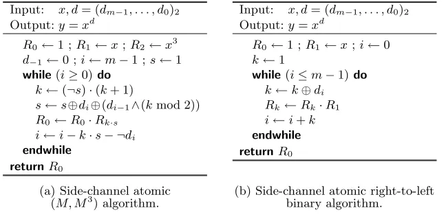
3.3 Simplified algorithms
Input: x, d= (dm−1, . . . , d0)2 Output:y=xd
R0←1 ;R1←x;R2←x 3
d−1←0 ;i←m−1 ;s←1 while(i≥0)do
k←(¬s)·(k+ 1)
s←s⊕di⊕(di−1∧(kmod 2)) R0←R0·Rk·s
i←i−k·s− ¬di endwhile
returnR0
Input: x, d= (dm−1, . . . , d0)2 Output:y=xd
R0←1 ;R1←x;i←0 k←1
while(i≤m−1)do k←k⊕di Rk←Rk·R1 i←i+k endwhile
returnR0
(a) Side-channel atomic (b) Side-channel atomic right-to-left (M, M3
) algorithm. binary algorithm.
Fig. 4.Further simplified algorithms for constrained devices.
referred to as the (M, M3) algorithm. The generic algorithm of Fig. 3 can then
be simplified to the algorithm given in Fig. 4-a.
In some cases, it is easier to scan bits from the least significant position to the most significant one. There is a right-to-left analogue of the square-and-multiply algorithm for computing y =xd. Analogously to Fig. 2, we can modify it into an algorithm preventing simple side-channel attacks. After simplification, we get the protected right-to-left exponentiation algorithm given in Fig. 4-b.
There are of course numerous possible variants that may be more efficient on a particular given architecture. What is remarkable is that our protected algorithms have roughly the same complexity (running time and memory re-quirements) as their respective unprotected versions.
4
Side-Channel Atomic Elliptic Curve Point
Multiplication
Our methodology applies to virtually any algorithm. We show hereafter how to adapt it in the context of elliptic curve cryptography [12]. Two categories of elliptic curves are commonly used [13]: elliptic curves over large prime fields and non-supersingular elliptic curves over binary fields. The basic operation in elliptic curve cryptography consists in computing the multiple of a point, that is, given a pointP1on an elliptic curve, one has to compute Pd =dP1. To ease
the presentation, we assume that this is carried out with the (additive version of the) square-and-multiply algorithm. Other methods are discussed in [14]. Our methodology readily applies to those implementation choices as well.
4.1 Elliptic curves defined over large prime fields
Consider the elliptic curveEdefined over a prime fieldFp(withp >3) given by
the Weierstraß equation
To avoid field inversion, Jacobian coordinates are generally used [13] for representing points on E. With Jacobian coordinates, the doubling of P1 is
2(X1, Y1, Z1) = (X3, Y3, Z3) where
X3=M2−2S, Y3=M(S−X3)−T, Z3= 2Y1Z1
with M = 3X2
1 +aZ14, S = 4X1Y12 and T = 8Y14. The sum of two (distinct)
pointsP1= (X1, Y1, Z1) andP2= (X2, Y2, Z2) is (X3, Y3, Z3) where
X3=W3−2U1W2+R2,
Y3=−S1W3+R(U1W2−X3), Z3=Z1Z2W
with U1 = X1Z22, U2 = X2Z12, S1 = Y1Z23, S2 = Y2Z13, W = U1−U2 and
R=S1−S2.
As the operations doubling or adding points are somewhat involved, we adopt the explicit approach. We refer the reader to the appendix for the detailed for-mulæ leading to the expression of atomic blocksγk as the rows of matrix:
(u∗
k,l)0≤k≤25 0≤l≤9
=
4 1 1 5 4 4 3 4 4 5 5 3 3 1 1 1 3 1 1 3 5 5 5 1 1 3 3 1 1 3 5 0 5 4 4 5 3 5 2 2 3 3 5 1 1 3 3 1 1 3 2 2 2 2 2 2 4 1 1 3 5 1 2 1 1 5 5 1 1 5 1 4 4 1 1 5 4 1 1 5 2 2 2 2 2 2 3 5 1 5 4 4 5 2 2 4 2 4 4 5 4 9 9 5 1 5 5 5 1 5 1 1 4 5 1 5 5 5 1 5 4 4 9 5 1 5 5 5 1 5 2 2 4 5 1 5 5 5 1 5 4 3 3 5 1 5 5 5 1 5 5 4 7 2 2 5 5 5 1 5 4 3 4 2 2 5 6 6 5 6 4 4 8 6 5 6 4 4 2 4 3 3 9 6 5 6 6 6 5 6 3 3 5 6 5 6 6 6 5 6 6 5 5 6 3 6 3 6 3 6 1 1 6 1 1 4 4 1 1 4 5 5 6 6 1 2 2 6 2 6 1 4 4 1 1 5 6 1 1 6 2 2 5 1 1 6 3 6 1 6 4 4 6 2 2 4 6 6 1 6
.
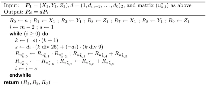
Input: P1= (X1, Y1, Z1), d= (1, dm−2, . . . , d0)2, and matrix (u∗k,l) as above Output:Pd=dP1
R0←a;R1←X1 ;R2←Y1;R3←Z1 ;R7←X1 ;R8←Y1 ;R9←Z1 i←m−2 ;s←1
while(i≥0)do k←(¬s)·(k+ 1)
s←di·(kdiv 25) + (¬di)·(kdiv 9) Ru∗
k,0 ←Ru∗k,1·Ru∗k,2 ;Ru∗k,3 ←Ru∗k,4+Ru∗k,5
Ru∗
k,6 ← −Ru∗k,6 ;Ru∗k,7←Ru∗k,8+Ru∗k,9
i←i−s endwhile
return(R1, R2, R3)
Fig. 5.Side-channel atomic double-and-add algorithm for elliptic curves overFp.
Again, it is worth noting that, in terms of field multiplications, this algorithm is as efficient as the corresponding unprotected implementation (cf. [13]).
4.2 Elliptic curves defined over a binary field
Atomicity is a relative notion. In the previous examples, we considered addition and multiplication as basic operations. One could also imagine that division is an basic operation; for instance, if division is provided by a dedicated hardware routine. The more different (from a side-channel perspective) basic operations there are, the more difficult it is to exhibit a common side-channel atomic block Γ. We give hereafter an example involving a division (a rather costly operation) as basic operation.
For efficiency reasons, it is recommended to use affine coordinates for adding points on an elliptic curve defined over a binary field [15]. A (non-supersingular) elliptic curve E defined over the binary field F2q is given by the Weierstraß
equation
E/F2q :y
2+xy=x3+ax2+b .
In affine coordinates (cf. [13]), the doubling of pointP1= (x1, y1) is 2(x1, y1) =
(x3, y3) where
x3=a+λ2+λ, y3= (x1+x3)λ+x3+y1
with λ = x1+ (y1/x1). The sum of two (distinct) points P1 = (x1, y1) and
P2= (x2, y2) is (x3, y3) where
x3=a+λ2+λ+x1+x2, y3= (x1+x3)λ+x3+y1
withλ= (y1+y2)/(x1+x2). We clearly see that doubling and addition of points
doubling or addition (see Fig. 6-a). Only two extra (field) additions are needed for doubling a point compared to the unprotected version of [13].
From this, an efficient protected double-and-add algorithm can then be de-rived (see Fig. 6-b).
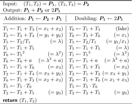
Input: (T1, T2) =P1, (T3, T4) =P2 Output:P1+P2or 2P1
Addition:P1←P2+P1 Doubling:P1←2P1
T1←T1+T3(=x1+x2) T6←T1+T3 (fake) T2←T2+T4 (=y1+y2) T6←T3+T6 (=x1) T5←T2/T1 (=λ) T5←T2/T1 (=y1/x1) T1←T1+T5 T5←T1+T5 (=λ) T6←T52 (=λ2) T1←T52 (=λ2) T6←T6+a (=λ2+a) T1←T1+a (=λ2+a) T1←T1+T6 (=x3) T1←T1+T5 (=x3) T2←T1+T4 (=x3+y2) T2←T1+T2 (=x3+y1) T6←T1+T3(=x2+x3) T6←T1+T6(=x1+x3) T5←T5·T6 T5←T5·T6
T2←T2+T5 (=y3) T2←T2+T5 (=y3) return(T1, T2)
Input: P1= (x1, y1), d= (1, dm−2, . . . , d0)2 Output:Pd=dP1
R1←x1 ;R2←y1 ;R3←x1 ;R4←y1 i←m−2 ;s←1
while(i≥0)do
k←(¬s)·(k+ 1) ;s←k∨(¬di)
R6−5k←R1+R3;R6−4k←R3−k+R6−2k R5←R2/R1
R5−4k←R1+R5 R1+5k←(R5)2 R1+5k←R1+5k+a R1←R1+R5+k
R2←R1+R2+2k;R6←R1+R6−3k R5←R5·R6 ;R2←R2+R5 i←i−s
endwhile
return(R1, R2)
(a) Side-channel atomic elliptic curve addition7
(b) Side-channel atomic double-and-add for elliptic curves overF2q. for elliptic curves overF2q.
Fig. 6.Side-channel atomic elliptic curve algorithms.
5
Conclusion
This paper introduced the notion of common side-channel atomicity. Based on this, novel solutions towards resistance against side-channel attacks were pre-sented. The proposed solutions are generic and apply to a large variety of cryp-tographic systems. In particular, they apply to exponentiation-based systems for which they lead to protected algorithms having roughly the same efficiency as their straightforward (i.e. unprotected) implementations. Finally, it should be noted that our methodology nicely combines with countermeasures against the more sophisticated differential analysis.
7
Acknowledgements
Part of this work was performed while the second author was visiting Gemplus. Thanks go to David Naccache, Philippe Proust and Jean-Jacques Quisquater for making this arrangement possible.
References
1. O. Goldreich.Foundations of Cryptography – Basic Tools. Cambridge University Press, 2001.
2. D. Boneh, R.A. DeMillo, and R.J. Lipton. On the importance of checking crypto-graphic protocols for faults. InAdvances in Cryptology – EUROCRYPT ’97, vol. 1233 ofLecture Notes in Computer Science, pages 37–51. Springer-Verlag, 1997. 3. P.C. Kocher. Timing attacks on implementations of Diffie-Hellman, RSA, DSS,
and other systems. InAdvances in Cryptology – CRYPTO ’96, vol. 1109 ofLecture Notes in Computer Science, pages 104–113. Springer-Verlag, 1996.
4. P.C. Kocher, J. Jaffe, and B. Jun. Differential power analysis. In Advances in Cryptology – CRYPTO ’99, vol. 1666 ofLecture Notes in Computer Science, pages 388–397. Springer-Verlag, 1999.
5. B. Chevallier-Mames and M. Joye. Proc´ed´e cryptographique prot´eg´e contre les attaques de type `a canal cach´e. Demande de brevet fran¸cais, FR 28 38 210, April 2002.
6. J.-S. Coron. Resistance against differential power analysis for elliptic curve cryp-tosystems. In Cryptographic Hardware and Embedded Systems (CHES ’99), vol. 1717 ofLecture Note in Computer Science, pages 292–302. Springer-Verlag, 1999. 7. R.L. Rivest, A. Shamir, and L.M. Adleman. A method for obtaining digital signa-tures and public-key cryptosystems.Communications of the ACM 21(2):120–126, 1976.
8. M. Joye. Recovering lost efficiency of exponentiation algorithms on smart cards.
Electronics Letters 38(19):1095–1097, 2002.
9. A.J. Menezes, P.C. van Oorschot, and S.A. Vanstone.Handbook of Applied Cryp-tography. CRC Press, 1997.
10. L.-C.-K. Hui and K.-Y. Lam. Fast square-and-multiply exponentiation for RSA.
Electronics Letters 30(17):1396–1397, 1994.
11. K.-Y. Lam and L.-C.-K. Hui. Efficiency ofSS(l) square-and-multiply exponenti-ation algorithms.Electronics Letters 30(25):2115–2116, 1994.
12. I. Blake, G. Seroussi, and N.P. Smart.Elliptic Curves in Cryptography. Cambridge University Press, 1999.
13. IEEE Std 1363-2000.IEEE Standard Specifications for Public-Key Cryptography. IEEE Computer Society, August 29, 2000.
14. D.M. Gordon. A survey of fast exponentiation methods. Journal of Algorithms
27:129–146, 1998.
15. E. De Win, S. Mister, B. Preneel, and M. Wiener.On the performance of signature schemes based on elliptic curves. InAlgorithmic Number Theory Symposium, vol. 1423 ofLecture Notes in Computer Science, pages 252–266. Springer-Verlag, 1998. 16. M. Joye and C. Tymen. Protections against differential analysis for elliptic curve cryptography: An algebraic approach. InCryptographic Hardware and Embedded Systems (CHES 2001), vol. 2162 of Lecture Notes in Computer Science, pages 377–390. Springer-Verlag, 2001.
17. C.D. Walter. MIST: An efficient randomized exponentiation algorithm for re-sisting power analysis. In Topics in Cryptology – CT-RSA 2002, vol. 2271 of of
A
Matrix Representation for the Side-Channel Atomic
Double-and-Add Algorithm for Elliptic Curves over
F
pThis appendix details how matrix (u∗
k,l) used in the double-and-add algorithm of Fig. 5 was obtained.
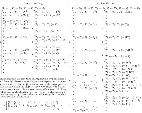
From the point addition formulæ given in Section 4.1, we see that doubling a point requires 10 multiplications and adding two points requires 16 multiplica-tions. In addition to multiplications, adding or doubling points also involve (field) additions/subtractions. Consequently, a common side-channel atomic block,Γ, must at least include one multiplication and one addition (a subtraction can be considered as a special case of negation followed by an addition). Since 1) the formula for adding two (distinct) points requires more multiplications than (field) additions, and 2) the formula for doubling a point requires 11 (field) additions/subtractions, we choose to expressΓ with 1 (field) multiplication and 2 (field) additions (along with a negation to possibly perform a subtraction).
We now express the point doubling and point addition as a repetition of blocks side-channel equivalent to Γ. A ‘?’ indicates that any register that does not disturb the course of the algorithm can be selected.
Replacing the ‘?’ by appropriate choices, processΠ0 (doubling followed by
an addition) and processΠ1(doubling) in the double-and-add algorithm can be
defined by matrix
(uk,l)0≤k≤35 0≤l≤10
=
4 1 1 5 4 4 3 4 4 5 0 5 3 3 1 1 1 3 1 1 3 0 5 5 5 1 1 3 3 1 1 3 0 5 0 5 4 4 5 3 5 2 2 0 3 3 5 1 1 3 3 1 1 3 0 2 2 2 2 2 2 4 1 1 3 0 5 1 2 1 1 5 5 1 1 5 0 1 4 4 1 1 5 4 1 1 5 0 2 2 2 2 2 2 3 5 1 5 0 4 4 5 2 2 4 2 4 4 5 0 4 9 9 5 1 5 5 5 1 5 0 1 1 4 5 1 5 5 5 1 5 0 4 4 9 5 1 5 5 5 1 5 0 2 2 4 5 1 5 5 5 1 5 0 4 3 3 5 1 5 5 5 1 5 0 5 4 7 2 2 5 5 5 1 5 0 4 3 4 2 2 5 6 6 5 6 0 4 4 8 6 5 6 4 4 2 4 0 3 3 9 6 5 6 6 6 5 6 0 3 3 5 6 5 6 6 6 5 6 0 6 5 5 6 3 6 3 6 3 6 0 1 1 6 1 1 4 4 1 1 4 0 5 5 6 6 1 2 2 6 2 6 0 1 4 4 1 1 5 6 1 1 6 0 2 2 5 1 1 6 3 6 1 6 0 4 4 6 2 2 4 6 6 1 6 1 4 1 1 5 4 4 3 4 4 5 0 5 3 3 1 1 1 3 1 1 3 0 5 5 5 1 1 3 3 1 1 3 0 5 0 5 4 4 5 3 5 2 2 0 3 3 5 1 1 3 3 1 1 3 0 2 2 2 2 2 2 4 1 1 3 0 5 1 2 1 1 5 5 1 1 5 0 1 4 4 1 1 5 4 1 1 5 0 2 2 2 2 2 2 3 5 1 5 0 4 4 5 2 2 4 2 4 4 5 1
Point doubling Point addition T0←a,T1←X1,T2←Y1,T3←Z1
1.
T4←T1·T1 (=X12) T5←T4+T4 (= 2X12) ?
T4←T4+T5 (= 3X12) 6.
T2←T2·T2 (=Y12) T2←T2+T2 (= 2Y12) ? ? 2.
T5←T3·T3 (=Z12) T1←T1+T1 (= 2X1) ? ? 7.
T5←T1·T2 (=S) ?
T5← −T5 (=−S) ? 3.
T5←T5·T5 (=Z14) ? ? ? 8.
T1←T4·T4 (=M2) T1←T1+T5 (=M2−S) ?
T1←T1+T5 (=X2)
4.
T5←T0·T5 (=aZ14) T4←T4+T5 (=M) ?
T5←T2+T2 (= 2Y1) 9.
T2←T2·T2 (= 4Y14) T2←T2+T2 (=T) ?
T5←T1+T5 (=X2−S)
5.
T3←T3·T5 (=Z2) ? ? ? 10.
T4←T4·T5 (=−Y2−T) T2←T2+T4 (=−Y2) T2← −T2 (=Y2) ?
These formulæ assume that multiplication by parametera (cf. Step 4) behaves identically as a multiplication with an-other value. If this multiplication can be distinguished by side-channel analysis, elliptic curve operations can be per-formed on a randomly chosen isomorphic curve [16]. Pro-vided that multiplication by−acannot be distinguished, another way to prevent side-channel leakage is to replace above Steps 2, 3 and 4 by
2.
T5←T3·T3
T1←T1+T1
T0← −T0
?
3.
T5←T5·T5
? T5← −T5
?
4.
T5←T0·T5
T4←T4+T5
T0← −T0
T5←T2+T2
.
T1←X1,T2←Y1,T3←Z1,T7←X2,T8←Y2,T9 ←Z2
1.
T4←T9·T9 (=Z22) ? ? ? 9.
T3←T3·T9 (=Z1Z2) ? ? ? 2.
T1←T1·T4 (=U1) ? ? ? 10.
T3←T3·T5 (=Z3) ? ? ? 3.
T4←T4·T9 (=Z23) ? ? ? 11.
T6←T5·T5 (=W2) ? ? ? 4.
T2←T2·T4 (=S1) ? ? ? 12.
T1←T1·T6 (=U1W2) ?
T4← −T4 (=−R) ? 5.
T4←T3·T3 (=Z12) ? ? ? 13.
T5←T5·T6 (=W3) T6←T1+T2(=S1+U1W2) T2← −T2 (=−S1) T6←T2+T6(=U1W2)
6.
T5←T4·T7 (=U2) ?
T5← −T5 (=−U2) T5←T1+T5(=W)
14.
T1←T4·T4 (=R2) T1←T1+T5(=R2+W3) T6← −T6 (=−U1W2) T1←T1+T6(=X3+U1W2)
7.
T4←T3·T4 (=Z13) ? ? ? 15.
T2←T2·T5 (=−S1W3) T1←T1+T6(=X3) ?
T6←T1+T6(=X3−U1W2)
8.
T4←T4·T8 (=S2) ?
T4← −T4 (−S2) T4←T2+T4(=R)
16.
T4←T4·T6 (=Y3+S1W3) T2←T2+T4(=Y3)
? ?
whosekthrow represents sequenceγ
k, which reads as γk = [Ruk,0 ←Ruk,1·Ruk,2;Ruk,3 ←Ruk,4+Ruk,5;
Ruk,6 ← −Ruk,6;Ruk,7 ←Ruk,8+Ruk,9;i←i−uk,10] .
So, a direct application yields the following implementation of the double-and-add algorithm.
Input: P1= (X1, Y1, Z1), d= (1, dm−2, . . . , d0)2, and matrix (uk,l) as above Output:Pd=dP1
R0←a;R1←X1 ;R2←Y1 ;R3←Z1 ;R7←X1 ;R8←Y1;R9←Z1 i←m−2 ;s←1
while(i≥0) do
k←(¬s)·(k+ 1) +s·26(¬di)
(u0, u1, . . . , u9, s)←(uk,0, uk,1, . . . , uk,9, uk,10)
Ru0←Ru1·Ru2 ;Ru3←Ru4+Ru5 ;Ru6← −Ru6 ;Ru7 ←Ru8+Ru9
i←i−s return(R1, R2, R3)
Fig. 8. A [simple] side-channel atomic double-and-add algorithm for elliptic curves overFp.
Matrix (uk,l) is highly redundant: except for variable s (last column), the first 10 rows are exactly the same as the last 10 ones. This is not too surprising since these rows correspond to the same operation (namely an elliptic curve doubling). It is fairly easy to remove the redundancy. Since, except fors, the 10 rows representing a doubling in matrix (uk,l) are equivalent, they can be shared. It suffices then to expresss as a function of di and k in the optimized matrix (u∗
k,l) given by
(u∗
k,l)0≤k≤25 0≤l≤9
=
4 1 1 5 4 4 3 4 4 5 5 3 3 1 1 1 3 1 1 3 5 5 5 1 1 3 3 1 1 3 5 0 5 4 4 5 3 5 2 2 3 3 5 1 1 3 3 1 1 3 2 2 2 2 2 2 4 1 1 3 5 1 2 1 1 5 5 1 1 5 1 4 4 1 1 5 4 1 1 5 2 2 2 2 2 2 3 5 1 5 4 4 5 2 2 4 2 4 4 5 4 9 9 5 1 5 5 5 1 5 1 1 4 5 1 5 5 5 1 5 4 4 9 5 1 5 5 5 1 5 2 2 4 5 1 5 5 5 1 5 4 3 3 5 1 5 5 5 1 5 5 4 7 2 2 5 5 5 1 5 4 3 4 2 2 5 6 6 5 6 4 4 8 6 5 6 4 4 2 4 3 3 9 6 5 6 6 6 5 6 3 3 5 6 5 6 6 6 5 6 6 5 5 6 3 6 3 6 3 6 1 1 6 1 1 4 4 1 1 4 5 5 6 6 1 2 2 6 2 6 1 4 4 1 1 5 6 1 1 6 2 2 5 1 1 6 3 6 1 6 4 4 6 2 2 4 6 6 1 6
Since, when di= 1 we haves= 0 if 0≤k≤24 ands= 1 ifk= 25, and when di= 0 we haves= 0 if 0≤k≤8 ands= 1 ifk= 9, we may for example define sas
s=di·(kdiv 25) + (¬di)·(kdiv 9) .
The expression forkmust also be modified accordingly:kis always incremented unless when s= 1, in which case it must be set to 0. So,k← (¬s)·(k+ 1) is a valid expression for updatingk. Doing so, we obtain the algorithm of Fig. 5, which is very similar to the one above but with a smaller matrix representation (i.e. matrix (u∗
k,l)).
B
Side-Channel Atomic Implementation of the MIST
Exponentiation Algorithm
MIST is a randomized exponentiation algorithm for preventing DPA-like attacks. However, as presented in [17], the MIST algorithm is susceptible to SPA-like analysis. We give hereafter a [simple] side-channel atomic version of the MIST algorithm8 as an additional illustration of the genericity of our methodoly for
preventing SPA-like attacks.
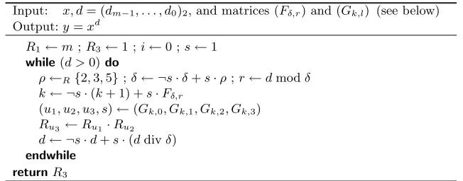
Input: x, d= (dm−1, . . . , d0)2, and matrices (Fδ,r) and (Gk,l) (see below) Output:y=xd
R1←m;R3←1 ;i←0 ;s←1 while(d >0)do
ρ←R{2,3,5};δ← ¬s·δ+s·ρ;r←dmodδ k← ¬s·(k+ 1) +s·Fδ,r
(u1, u2, u3, s)←(Gk,0, Gk,1, Gk,2, Gk,3) Ru3 ←Ru1·Ru2
d← ¬s·d+s·(ddivδ) endwhile
returnR3
Fig. 9.Side-channel atomic MIST exponentiation algorithm.9
8
To avoid register rewritting, the divisor subchain corresponding to the divi-sor/residue pair [2,1] is replaced with{(133),(111)}. The original MIST algorithm uses subchain{(112),(133)}; cf. [17, Table 3.1].
9
with matrices:
(Fδ,r)2≤δ≤5 0≤r≤4
=
0 1 ? ? ? 3 5 8 ? ? ? ? ? ? ? 11 14 18 22 26
and (Gk,l)0≤k≤29 0≤l≤4
=
1 1 1 1 1 3 3 0 1 1 1 1 1 1 2 0 1 2 1 1 1 1 2 0 1 3 3 0 1 2 1 1 1 1 2 0 2 3 3 0 1 2 1 1 1 1 2 0 1 2 1 0 1 2 1 1 1 1 2 0 1 3 3 0 1 2 1 0 1 2 1 1 1 1 2 0 2 3 3 0 1 2 1 0 1 2 1 1 1 1 2 0 1 2 1 0 1 3 3 0 1 2 1 1 1 1 2 0 2 2 2 0 2 3 3 0 1 2 1 1

![Fig. 8. A [simple] side-channel atomic double-and-add algorithm for elliptic curvesover Fp.](https://thumb-us.123doks.com/thumbv2/123dok_us/1839786.1238325/14.595.144.472.218.334/fig-simple-channel-atomic-double-algorithm-elliptic-curvesover.webp)