DISTRIBUTION OF GENE FREQUENCY AS A TEST OF THE THEORY OF THE SELECTIVE NEUTRALITY OF POLYMORPHISMS

DISTRIBUTION

OF

GENE FREQUENCY

AS A

TEST

OF

THE THEORY O F THE SELECTIVE NEUTRALITY OF

POLYMORPHISMSJ

R. C. LEWONTIN A N D JESSE KRAKAUER Department of Thoretical Biology and Department of Biology,

University of Chicago, Chicago, Illinois 60637

Manuscript received February 14, 1972 Revised copy received January 16, 1973

Transmitted by T. PROUT

ABSTRACT

The variation in gene frequency among populations or between generations within a population is a result of breeding structure and selection. But breeding structure should affect all loci and alleles in the same way. If there is signifi- cant heterogeneity between loci in their apparent inbreeding coefficients P = s p 2 / p (1 -p), this heterogeneity may be taken as evidence for selection. We

have given the statistical properties of F and shown how tests of heterogeneity can be made. Using data from human populations we have shown highly significant heterogeneity in F values for human polymorphic genes over the world, thus demonstrating that a significant fraction of human polymorphisms owe their current gene frequencies to the action of natural selection. We have also applied the method to temporal variation within a population f o r data o n

Dacus oleae and have found no significant evidence of selection.

HE discovery of vast amounts of polymorphism in sexually reproducing ani-

Tmals and plants since the first reports by HARRIS, by

HUBBY

and LEWONTIN

and by

JOHNSON

et al. in 1966, has given a considerable impetus to the problem

of distinguishing between natural selection and essentially non-selective proc-

esses, such as restriction of population size, recurrent mutation and migration,

on the determination of genetic variation. A synthetic view does not allow an

“either-or” approach to this problem, but admits that gene frequency distribu-

tions are the result of the interaction of selective and non-selective forces. Yet

even in such a view there exists the strong possibility that selection coefficients are of such a magnitude for most genes that variations

in

time and space and between loci in the array of allele frequencies can be explained in large part without reference to variation in selection coefficients. That is, in the sense of the analysis of variance, the main effect of selection in determining gene fre- quencies is small.

One of the main problems of assessing the role of natural selection lies in the

This paper is dedicated to the memory of Ken-ichi Kojima, who was killed in the full flood of his life on November 14,

1971. He was a n imaginative scientist who made many important contributions to evolutionary genetics, and h e was a

dear friend.

176 R. C . LEWONTIN A N D J. IIRAKAUER

probable size of selection coefficients. Even the most sanguine “selectionist” will not claim that selection coefficients in excess of a few percent are the rule. But the power to detect selection of this magnitude by observing changes in gene fre-

quency, or differences in components of fitness between genotypes, is very low

for sample sizes within the range of practicality (see WILSON 1970, for a gen-

eral theoretical treatment of the estimation problem, and

YAMAZAKI

1971, for a

specific example in an experimental context). The alternative is then to use in- formation about the spatio-temporal distribution of allelic frequencies on the assumption that these frequencies are in a steady-state distribution resulting from the interaction of the various forces, and so attempt, from the distribution, to

estimate the forces. The difficulty with this procedure is that various parameters

enter in a confounded way into the determination of the observations. For exam-

ple, the steady-state distribution of allelic frequencies over populations depends

critically on terms such as N s and

N

( p + n ) where s is the intensity of selection,

p the mutation rate to one of the alleles, m the migration rate from neighboring

populations (in the extremely simplified model of island populations) and

N ,

the

effective population size, a number only loosely related to census size. Not only

is selection confounded with the other parameters, but those parameters are ex-

tremely difficult to measure in practice. Measurements of either migration rates or effective population sizes are, both practical and conceptual reasons, virtually

impossible-especially if populations do not conform to simple “island” struc-

ture, and intuitive notions about whether N is Very large” or m is “small enough

to be ignored” are useless, especially in view of the fact that these two parameters appear as their product, N m , in the theory! So, any observed distribution of gene frequencies over space or time, if considered to be in a steady state can be ex- plained by a suitable choice of

N ,

m and p , with s being made arbitrarily small,

the more so because the number of populations or time points observed is never

really very large and the distribution is poorly known. As an example, PRAKASH,

LEWONTIN and

HUBBY

(1969) showed that the allelic frequencies at 24 loci, 11 of

which were polymorphic, were very similar in three widely separated popula-

tions of Drosophila pseudoobscura, and recent, as yet unpublished, work from

the same laboratory extends these similarities to a half dozen more such popula- tions. One explanation of the striking similarity of allelic frequencies among

populations 2000 miles apart, even for loci with five to eight alleles segregating,

is that these frequencies are in stable equilibrium held by common selective forces in all populations. An equally good fit to the data, however, can be made by the hypothesis that there is no selection and that effective migration over the range of the species is of the order of one individual per generation between

neighboring populations (WRIGHT 1951). It is impossible to rule out, by direct

evidence, migration rates of that order. (Even allelism of lethals between popula-

tions is totally insensitive to small migration rates).

What is required is some method of detecting selection which will cancel out the effects of the breeding structure. In principle, such a method is possible be-

cause there is one feature of migration, genetic drift and inbreeding that is quite

TEST O F SELECTIVE NEUTRALITY THEORY 177

locus and each aZleZe at a locus, the effect of breeding structure is uniform over all loci and all alleles. Inbreeding affects all genes simultaneously and to the same average degree, as does sampling variation and migration. In the absence of selec- tion, the steady-state variation in frequency of an allele at a locus from popula- tion t o population, or from time to time, is entirely a reflection of the breeding structure of the species and, in fact, the variation of frequency can be used to esti-

mate a parameter Fe, the “effective inbreeding coefficient” for the collection of

populations. The effective inbreeding coefficient is a kind of fictitious equivalent to the inbreeding coefficient that would arise after some fixed number of genera- tions in a model of totally isolated populations with no migration between them,

perfect panmixia within them, each of a constant size

N ,

that would produce the

amount of genetic variation observed among the real populations. The fact that the real populations do exchange genes, do fluctuate in size and are not perfectly panmictic is irrelevant, because these actual conditions are summarized in the

“effective” parameter Fe, which has no interest in itself. The estimate is simply

where

E ,

= estimate of effective inbreeding,

sZp = variance in the frequency of one of two alternate alleles from

p

= mean frequency of the allele over the ensemble of populations.

population to population, and

Now suppose we carry out the estimate in using a number of different loci, each of which will have its own values of szp and

p .

If

all these loci are selectively

neutral, they will all estimate the same Fe since the estimations apply to all genes

in the ensemble of populations. Then the collection of

E ,

values actually calcu-

lated will be an estimation of a true Fe and there should be no significant hetero-

geneity among them. On the other hand, if some or all of the loci are under se-

lection, the various Fe’s will not be estimates of the same

Fe

because they will be distorted by selection. For the selection loci the .Pp values and therefore the esti- mated E , will be too large if selection is different in different populations, while if there is a selection in common, the variance among populations will be too small. Even if all the loci are under some selection, the

P ,

will not be drawn from the same distribution unless selection is acting identically over all alleles. This

idea was first used, as far as we know, by CAVALLI-SFORZA (1966), who calcu-

lated E , values over a wide range of human groups encompassing the diversity of

the species, f o r fifteen different gene frequencies, representing nine loci. The

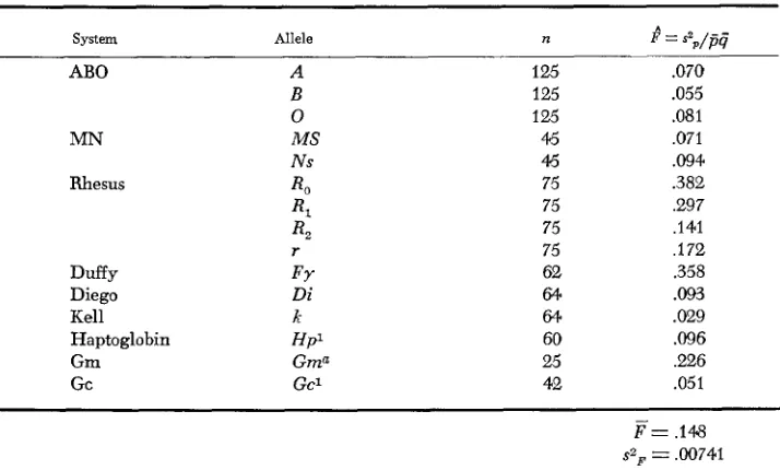
values of E , from CAVALLI-SFORZA are reproduced as Table 1 of this paper. The

considerable variation in E , values from .029 for the Kell blood group locus, to

.382 for the R, allele of the Rh locus seemed to CAVALLI-SFORZA as too great to ex- plain from sampling error alone, but that impression could not be tested in the absence of any sampling theory. We shall return to the data of Table 1 later.

In principle, then, a test of the homogeneity of E , estimates derived from dif- ferent loci in steady state will be a test of the homogeneity of selection coefficients across loci-which, in effect, is a test for selection. In practice, the problem is to

178 R. C. LEWONTIN A N D J . KRAKAUER

TABLE 1

I? values for world wide distribution of h u m polymorphisms. n is the number

of groups sampled. Data from CAVALLI-SFORZA (1966)

system Allele n L s 2 / - - P P9

AB0

MN

Rhesus

Duffy Diego Kell Haptoglobin Gm Gc

125 125 125

45

45

75 75 75 75 62

64 64

60 25 42

.070 .055 .081 ,071 .094 .382 ,297 ,141 ,172 .358

.093

.a29

.096

,226 .051

F=

,148

sZF = ,00741

same universe and then to use this sampling distribution to test the significance

of the difference between two o r more

13,

values from different loci.

TWO MODELS

1. Variation in space: Let us postulate a locus with two alleles. A and a segregat- ing (or fixed) in a large number of populations. The populations are defined simply as sampling units and we know nothing about their actual breeding struc- ture or their degree of isolation from each other. Let pi be the frequency of allele

A in the itn population. Let us suppose we choose a random subset of n popula-

tions from the entire ensemble and determine the gene frequency pi in each. We

will further suppose that the determination of p i in each population is based upon sufficient sample size so that the within-population sampling variance is negli-

gible compared with variance among populations. That is, we know each pi to a

first approximation. If we then take the sample variances among the n values of

p i , and the mean,

p ,

we can calculate one estimate

From another subset of n randomly-chosen populations we can calculate another

value of P , and so on. Then the values of P , will have a distribution that depends upon the true variance of the pi, u Z p and the true mean, b. Unfortunately it

depends upon not just these two first moments, but also on the entire distribution

T E S T O F SELECTIVE N E U T R A L I T Y T H E O R Y 179

off on both sides, J-shaped, U-shaped or rectangular, depending upon the under-

lying parameters N , my s, etc. which are unknown. Nor can we estimate the form

of the distribution directly since we usually cannot sample enough populations to get a picture of it. In practice, of course, the sampling distribution of B might be rather insensitive to different shapes and, in the best of all possible worlds might depend only on the ratio ~ ~( 1 -&) ~

,

i.e., on the true value of / p ~ F . As we will show, for a given general functional form of the parent distribution of p i ,

the sampling distribution of B does depend only on the ratio d / p P ( l-pp)

,

that is,

on the true value of F; but when we change the form of the parent distribution,

the sampling distribution changes non-trivially. This latter, unfortunate fact,

leads us to consider an alternate procedure, origmally conceived of by C. KRIM-

BAS and actually utilized by KRIMBAS and TSAKAS (1971).

2.

Variation in time:

If

we observe the frequency of an allele in two successive generations in a population, and if that gene is not subject to natural selection, there will still be a change in the gene frequency, ~ p , because of the finite size of the population. If there were a very large number of identical populations all starting with the same gene frequency, there would be a variation in gene fre- quency among the populations after one generation which would be related to a n effective inbreeding coefficient by equation 1. W e will denote the inbreeding coefficient that arises after a single generation of such drift by f to distinguish it from the result of many generations of the process, Fe. The change, A p , within any single population can be used to estimate the variance among the populations and in fact

is a n estimate of the variance with one degree of freedom. Then a n estimate o f f is, from (1) and (2)

s2 = ( A p ) (2)

where p o is the gene frequency in the initial generation. If this is done for many different genes in the same population, then each such estimate, under the hy- pothesis of no selection, estimates the same true f, and we may apply the same reasoning as for

F.

The advantage of f over

E ,

however, is that we know the un- derlying distribution of the pi. It must be binomial3 with mean p o and variance

p o ( l - p O ) , because it is a one-stage sample of size 2Ne from a population with 2No

value po. We are not, in this case, plagued with the problem of the unknown un-

derlying gene frequency distribution that affects the sampling distribution of

P .

As we shall see, this is a particularly felicitous choice of a n underlying distribu- tion.

THE S A M P L I N G DISTRIBUTION O F

W e wish to find the distribution of the statistic

180 R. C . LEWONTIN AND J . KRAKAUER

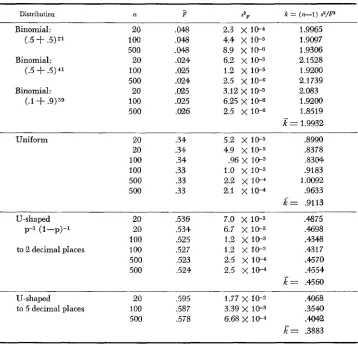
TABLE 2

Statistical of the empirical distributions of $ for different underlying distributions of p. n is the

variance and k = (n-I) $/F*

sample size on which each I? value is calculated, the mean, s2F the

Distribution n 3 ."I? k = (n-1) 52/F

Binomial: (.5

'+

.5) 2 1

Binomial: (.5

+

.5) 41

Binomial:

( A ' + .9)39

20 100 500 20 100 500 20 100 500 .048 ,048 .048 .024 .025 .U24 .025 .025 ,026

2.3 x 1W

8.9 x 10-6 4.4 x 10-5

6.2

x

1 0 - 5 1.2 x 1 e 5 2.5 x 10-6 3.12 x 1 ~ 5 6.25 x 1 0 - 6 2.5

x

10-6

k

1.9965 1.9097 1.9306 2.1 528 1.9200

2.1 739 2.083 1.9200 1.8519 = 1.9932

Uniform 20 .34 5.2 x 10-3 3990

20 .34 4.9 x 113-3 A378 100 .34 .96 x 10-3 .83W 100 .33 1.0

x

10-3 .9183 500 .33 2.2 x 10-4 1.0092 500 .33 2.1

x

10-4 .9633

k =

.9113

U-shaped 20 ,536 7.0 X 1 0 - 3 .4875

p-1 ( 1 -p) -1 20 .534 6.7 x 10-3 ,4698 100 .525 1.2 x le3 .4348 to 2 decimal places la0 .527 1.2 x 10-3 .4317 500 ,523 2.5 x 1w .4570 501) .524 2.5

x

10-4 .4554

x=

.%60

U-shaped 20 ,595 1.77 X .4068

to 5 decimal places 100 ,587 3.39 x 10-3 .3540 500 .578 6.68 X l e 4 .*2

t?= .3883

given that p has some specified distribution among populations and that s2p and j j

have been calculated from a sample of n populations. If the p i were very close to being normally distributed, and if n were large enough s3 that jj were very close

to the true mean of p , then ( n - - l ) P / F would be very close to a chi-square distri-

bution with n-1 degrees of freedom. In actual fact, however, will vary around

the true mean and the distribution of p i will never really be normal, so we do not

know, a priori, how useful the chi-square distribution may be. The problems of

finding the distribution of

P

analytically seem to us formidable, in general, and

even if found would certainly require numerical tabulation; so we have used

TEST O F SELECTIVE NEUTRALITY THEORY 181

and the cumulative probabilities of observing a p less than or equal to that value.

A

random number from a uniform distribution on the interval [0, I], is then

generated and used to pick out a p value. This technique will choose p values in

proportion to the probabilities given by the postulated distribution. A sample of

n such p values is chosen and from this sample a single value of

E

is calculated

according to formula 1. The sampling cycle is repeated 5000 times to produce

5000

P

values which then represent an empirically derived sample distribution of

E,

given the hypothetical underlying distribution of p .

Table 2 shows the results of the simulations for underlying distribution of

p

that are binomial, flat, or U-shaped, corresponding to common distributions ex-

pected for steady state gene frequency distributions without selection. Both a symmetrical and an asymmetrical binomial distribution and two different vari- ances

( N

= 21 and N = 41) were tested. Two replicates for each of the uniform and U-shaped distributions are given, to show the reliability of the empirical statistics.

For the binomial distributions we see that the mean value of

E

is unaffected by

the asymmetry so that the normalizing effect of dividing the variance in gene

frequency by p(1-p) does indeed work. Moreover, the mean

P

turns out to be

very close to 1/21 = .0476 and 1/41 = .0244, that is to 1/N, which is exactly

what the expected value would be if the denominator of F,jj(I-jj), had no sam-

pling variance. In fact

s

turns out to be slightly greater than 1/N as a result of

the small sampling variance of the denominator, The mean value for the uni-

form distribution also turns out to be very close to the expected value of 4/12,

which would be the case if the denominator had no variance. For the U-shaped distribution it is more difficult to compare the observed mean with the ideal since the expectation depends critically on what convention is made concerning the

terminal classes. Obviously p=O and p=l must be excluded or the mean will be

infinite. The more finely-divided the underlying discrete distribution is, the

smaller the value of p in the subterminal classes and so the larger the value of F

since

p

appears in the denominator. Table 2 shows that an increase of the fineness of subdivision from 2 to

5

decimal places of the U-shaped distribution classes in- creases the value of

P

by about 15%.

If the distribution of F is in some sense invariant under changes in the pa-

rameters of the underlying distribution, there should be a relation between

r;;

and

sZF. In any case, s2F shoud be inversely proportional to (n-I), the degrees of freedom of

8,

and in addition if the distribution of

P

is invariant, we might guess that the variance of E will be proportional to

fi.

That is

In the last column of Table 2 we have calculated k = (n-1) s 2 / p f o r each run.

We see that for each form of distribution there is a characteristic k, and that for

the binomial distributions, k=2, irrespective of the parameters of the binomial.

This value for k is not coincidental. We remarked before that we expected that F

182 R . C. LEWONTIN A N D J. KRAKAUER

roughly normal. If p is binomial, then as noted by WORKMAN and NISWANDER

( 1 9 7 0 ) , the weighted sum of squares of the p i divided by jj ( 1 - j j ) is algebraically identical to the usual homogeneity statistic calculated from 2 x n tables. In par-

ticular

xz

is distributed with mean n-1 and variance 2(n-1) where n-1 is the

( n - l ) P

F

number of degrees of freedom. Now P has a mean

E

so will also have

a mean of (n-1 )

.

What will its variance be? It will be

-

(n-1)Z S 2 F

22

But we have shown in Table 2 that

(n-1 ) szF

P

_ _ ~- 2

-(n-1)P F

so the variance of

-__

will be 2 (n-I)

,

the same as the chi-square distribu-

(n-1)P

tim. I t would appear likely then that is distributed as

x 2

with n-1 de-

F

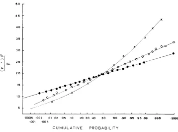
grees of freedom. To make a closer check, the empirical cumulative distribution of P is plotted in Figure 1 for several of the cases given in Table 2. The coordi-

nates of the abscissa are so arranged that a normally distributed variable will ap-

pear as a straight line with a slope equal to its standard deviation. Plotted on this

graph are the

P

distributions based on underlying binomial, uniform and

(n-l)P

U-shaped distributions. In each case the ordinate is in units of -

.

For the

F (n-1)F

are very

F

U-shaped and flat underlying distributions, the distribution of

.-

close to normal with mean n-1 and standard deviation .\/k(n-1) were

k

is given

in Table 2. On the other hand, the

P

distribution based on the binomial distribu-

tion deviates significantly from the normal, being concave upwards. This con- cavity means that the distribution is skewed to the left, in excellent agreement with the xZl9 distribution shown by the curved line. I t should be noted that this

curve is in no way “fitted” to the data.

It

is simply the chi-square distribution

with 19 degrees of freedom.

We may summarize the results of these empirical distribution studies as fol- lows. If the underlying distribution of gene frequencies across populations is

binomial or normal, then is distributed as x2 with n-1 degrees of free-

dom were n is the number of populations sampled. If the underlying distribution

of gene frequencies is much more dispersed than the binomial, then ___- is

normally distributed with mean (n-1) and a variance between a quarter and a

half of that for the binomial case. This latter point-that greater dispersion of

the underlying gene frequencies reduces the variance of P-will be extremely

important for testing hypotheses about the homogeneity of F values.

(n-1)P

-

F

TEST O F SELECTIVE NEUTRALITY THEORY 183

4 5 = O

1

4 0 35

t

5 1

J

0005 002 01 02 0 5 10 20 3 0 40 6 0 80 9 0 9 5 98 99 998 9999 0 0 1 0 0 5

C U M U L A T I V E P R O B A B I L I T Y

FIGURE 1 .-Empirical cumulative distributions of P given various underlying distributions of p . Abscissa is in units of probability on a scale arranged to produce a straight line if the distri- bution is normal. Ordinate in units of ( n - I )

k/g

Crosses: binomial; solid circles: uniform; open circles: U-shaped.

APPLICATION T O SPATIAL VARIATION

In 1966 ARENDS et al. published the distribution of 22 allelic frequencies be-

longing to 15 different loci, distributed over 10 villages of the Yanomama tribe

of Indians in the Orinoco Basin. These villages are partially isolated, but do ex-

change genes, and some villages have been formed from others by a process of

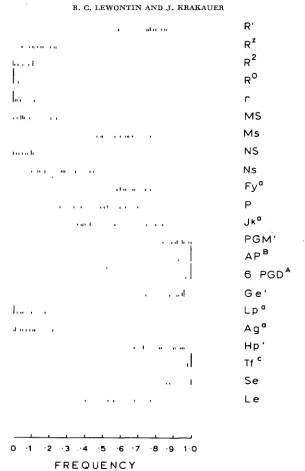
budding. Figure 2 shows the distribution of allelic frequencies among the villages

for the alleles investigated.

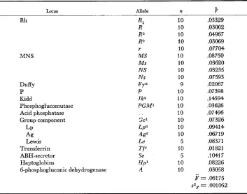
Table 3 gives the P value for each allele together with the number of villages

over which it has been estimated. The P values seem to fall in two groups, nine

of them being .036 or less and eleven being greater than .072, with only two be-

ing in between these groups. W e wish to test the hypothesis that this apparent heterogeneity of

P

values is real. The

P

values observed do not need to be cor- rected for sampling error within villages since, although the numbers in each vil- lage are small, they are nearly complete censuses rather than samples.

Based on our Monte Carlo results we could take two approaches. One would be to test the goodness of fit of the observed distribution of P values t o one of the

sampling distributions. Figure 2 shows that the underlying distribution of p f o r

184 R . C. LEWONTIN A N D J. K R A K A U E R

R 2

R0

I I *, I , . , .

II

I

r

MS

Ms

NS

N s

F Y

J k 0

P

P G M '

AP

6 PGDA

G e '

L P O

A g O

H P '

Tf

S e

L e

F R E Q U E N C Y

FIGURE 2.-Distribution of allelic frequencies f o r genetic systems of Table 3. Data from ARENDS et al. (1966).

unimodal binomial distribution. W e might then test the goodness of fit of the observed distribution of

E

values to a

x 2

distribution with nine degrees of freedom

(ten villages). Table

4

shows a comparison between the observed distribution of

TEST O F SELECTIVE NEUTRALITY THEORY

TABLE 3

185

k

values for diflerent allelic distributions among ten villages of Y a n o m m Indians n is the number of villages for each

6.

Calculated f r o m data of ARENDS et al. (1966)

Locus Allele n 9

Rh MNS Duffy P Kidd Phosphoglucomutase Acid phosphatase Group component LP Ag Lewis Transferrin ABH-secretor Haptoglobins 6-phosphogluconic dehydrogenase

10 .(I3329 10 .03002 10 ,04967 10 .03069 10 .077M 10 .08750 10 .03620 10 .03235 10 .a7593 9 .02067

10 .(I7398

10 .I4594 10 .03626 10 ,07496

10 .a7326 10 .OQ414 10 .06719

5 ,08371 10 .a1821 5 .1G417 10 .08226 10 .03058 = .MI75 s z p = .001052

TABLE 4

Comparison of the distribution of

fi

values of Table 3 and the theoretical x2 distribution

~

R

~

Observed Expected

.01372-,02744 .02745-.04116 ,041 17-.a5488 .05489-.06860 .06861-,08238 .08233-.09574

186 R. C. LEWONTIN A N D

J.

KRAKAUER

ard deviation of the

x2

distribution wide, centering on the observed mean F of

.06175. The test for goodness of a fit between the observed distribution and the

theoretical gave a

x2

= 13.41 with five degrees of freedom corresponding to

P = .02, so we judge the observed distribution of

P

to be significantly different from the theoretical sampling distribution. This difference results from the greater heterogeneity of the observed P , as evidenced in the two modes and is taken as evidence for selection on some of the genes. Of course we cannot tell whether the lower mode is the non-selected group, with diversifying selection accounting for the upper mode, or whether the lower mode is evidence f o r a com- mon heterotic selection acting over all villages.

A second test of heterogeneity would be the comparison of the observed vari- ance of

P

with the theoretical variance. As we have seen, the theoretical variance of

P

is given by

with

k=2

when the underlying distribution of p is binomial. Applying this rule

to the data of Table 3 we have

W e can test whether the observed variance szp = .001052 is significantly larger

by the ratio szF/uZ = 1.380 which will be distributed as x2/d.f. I n the analysis, there is a problem of what to do with the two multiple allelic systems, Rh and MNS. The variations in the various alleles at one locus are obviously correlated positively. That is, if one allele is very uniform over villages, other alleles must also tend to be uniform. To choose only one of the alleles arbitrarily, say the one closest to a frequency of

.5,

o r to average F values over alleles at one locus would be to sacrifice information. The effect of using this correlated information will be to overestimate the power of any test because of spurious degrees of freedom. We will compensate for this by removing one degree of freedom for each multi- ple allelic locus. This would be exactly correct in the case where both alleles at a di-allelic locus were used, and must be nearly so here, since each degree of free-

dom corresponds to a n added linear restriction on the ensemble of P values. In

this particular case, the number of degrees of freedom is then 22

-

3 = 19 and the probability of the ratio is P = .12, so the difference is not significant. The

ratio of variances has then failed to detect the excess heterogeneity of

P

values

shown from the goodness of fit test, which itself was significant only at the .02 level. Clearly the conclusions about heterogeneity of the P values is doubtful.

A fortunate circumstance makes it possible to perform a second test of this case. After these calculations were made, the Michigan group published more com-

plete data on the Yanomama for 16 of the original 22 allelic frequencies pIus a

new system, Diego. The 10 original villages plus 27 new ones are included in this new study, and the authors have also calculated P values f o r the different systems

(GERSHOWITZ et al. 1972; WEITKAMP et al. 1972; NEEL, WARD and MACCLUER

1972). This new study shows that the P values f o r the Yanomama are indeed

homogeneous since:

u 2 = .0007624

.

TEST O F SELECTIVE NEUTRALITY THEORY 187

2) There is no correlation between

E

values on the ten villages and E values

from the larger sample.

3) The ratio of observed variance of

P

to expected variance in the larger study

is .00413/.000216 = 1.55, which is referred t o the x2/d.f. distribution with 17 - 3 = 14 degrees of freedom and has a P = .IO.

Apparently, then, if selection is operating on the genes in the study, the villages are insufficiently isolated or too recent historically, to make detection possible.

What of the data in Table 1 for the worldwide distribution of gene frequencies? Here the underlying distribution of various gene frequencies is more problematic,

since some are close enough to binomial, but others with very high F values are

much closer to uniform or even U-shaped distributions on a world-wide basis. However, since the expected variance of

P

is smaller

( k

is smaller) for these un- derlying distributions than for the binomial, we can perform a conservative test

by using

k

= 2.0. The number of racial groups vanes in Table 1 from 25 to 125,

SO we have used the harmonic mean, 60, for n. The theoretical variance of the

P

for this case is then

= .000742

2.0 (.148)z

59 u 2

while the observed variance is .007416, so we have s 2 / d = 10.

Again subtracting a degree of freedom for each multiple allelic loci, we com- pare this ratio with the distribution of x2/d.f. f o r 11 degrees of freedom and obtain

a P

<

.001. Thus CAVALLI-SFORZA’S suggestion that the values are much too

heterogeneous to be explained without selection is amply justified. I n this case there is even some suggestion of which sort of selection has operated. On a world- wide basis, the most deviant allelic frequencies are generally found in groups

that have small populations and are isolated culturally and genetically from

other human groups. These include Eskimos, American Indians, Basques and Australian Aborigines, among others. There is no reason to suppose that natural selection will vary more between, say, American Indians and Australian Abo- rigines, both Stone Age peoples up until recently, than between, say, Europeans and Africans. Thus it is probably their isolation and small population size that has caused the divergence of these isolated groups. Then it is among the gene

frequencies that have not diverged, those associated with small F values, that we

should look for selection. In particular we should look for heterotic selection tend-

ing to retard divergence among the isolated groups with respect to these loci.

Both sets of human data differ in a significant way from the Monte Carlo

sampling scheme on which the distribution of

E

is based. For the Yanomama and

188 R. C . LEWONTIN A N D J. KRAKAUER

related than between races, Even the Yanomama villages are hierarchically re- lated because some have budded off from others in recent times. To see the effect of repeated sampling in a hierarchically-arranged set of populations, we consider the most extreme possible case of two genetically differentiated races, but with

all local populations within races identical. If we sample, say ten populations in

each race and calculate

P

for many loci, we have really sampled only two dif-

ferent populations, since there is no component of variation within races. Then

the appropriate value of n-I in the denominator of the theoretical variance of F

is only one instead of nineteen. However, compensating for this inflation of uz by the reduction of n is a reduction in the theoretical variance because of the re- peated samples from the same of set of populations. The underlying distribution of allele frequencies in this extreme case is bimodal, with half the populations having one allele frequency and the other half having a different frequency. But we are always choosing one “population” from each mode, whereas in a random sampling scheme we would by chance choose both populations from the same mode half the time. Thus, there are two opposite tendencies acting on the theo-

retical variance of

I3

when repeated samples are taken from the same set of hier-

archically-related populations, and we do not know the exact effect of these tendencies since we have not simulated this sampling scheme. For the Yanomama Indians, where the heterogeneity of

E

is o n the borderline of significance, we will

be made even more cautious. The observed variance for the world

E

values is,

however, so much greater than the theoretical variance that it is most unlikely that the altered sampling scheme has much effect.

THE S A M P L I N G DISTRIBUTION O F f

Because the use of the temporal inbreeding,

1,

will often involve multiple al-

lelic loci, we have simulated temporal sampling at a three-allele locus to deter- mine the effect of the correlation between allelic frequencies. Three initial fre-

quencies at the locus were specified and a random sample of

N

genes were taken

to form a new population. The changes in allele frequency, Apl, Ap,, and A p s ,

were then used to calculate

j

from the relation

This calculation was replicated 5000 times for each original distribution of p i

and for each population size

N .

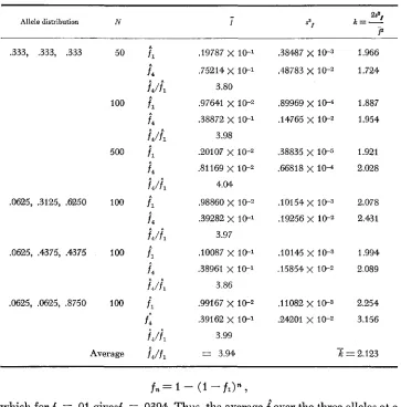
For each replicate, the simulation was pushed further. Because in nature it is often impossible to get gene frequency data every generation, the sampling scheme was carried out for four generations to check that f^ after four generations is essentially four times f after a single generation, as it should be for low levels of inbreeding. Table 5 gives the statistics of these runs in the same form as for Table 2. I t should be remembered that for all these runs, n = 3 since there are only three Ap’s that enter into each f calculation.

We see from Table

5

that each of the fl values is almost precisely 1/N and that

TEST O F SELECTIVE NEUTRALITY THEORY

TABLE 5

Statistics for the empirical distribution of

f^

for different initial gene frequency distributions. N is

the number o f genes in the brccding population (=2N,), f, is the single generution f

value, fi is the four generution value

189

*

Allele distribution N

.333, .333, .333 50

100

500

.0625, .3125, .6%0 100

.0625, .4375, .4375 100

.0625, .0625, .8750 100

Average

-

f

,19787 X I t 1 .75214

x

I t 1

3.80

.97641 X 10-2 .38872 X 10-1

3.98

,20107

x

10-2

.81169 x 10-2

4.04

.98860

x

10-2

.39282

x

10-1

3.97

.IO087 x 10-1

.38961

x

10-1

3.86

.99167

x

10-2

,39162

x

10-1

3.99

= 3.94

.38487

x

I t 3

,48783

x

le2

.89969 X 10-4 .I4765 X le2

,38835

x

I W

.66818

x

10-4

.IO154 X IW3 .I9256 X le2

.lo145 X 10-3 ,15854 x 10-2

. i m 2

x

l o r 3

.24201 X IOW

1.966

1.724

1.887

1.954

1.921

2.028

2.078

2.431

1.994

2.089

2.254

3.156

-

k = 2.1w

fn = 1

-

( 1

-

f l ) " ,

which for fl = .01 givesf, = .0394. Thus, the average

f^

over the three alleles at a tri-allelic locus is behaving exactly according to the theory for a single allele, as it

should. The average

IC

value is 2.123 and given the large variation from run to

run and the lack of pattern of these variations, the agreement with a value of 2.0

for the

x 2

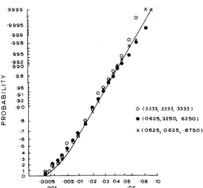
distribution is good, Indeed, nearly the whole excess over 2.0 is a result

of the very extreme value in the last run in the table. Figure 3 shows the cumu-

lative frequency distribution for several cases as compared with a x2 distribution

(corrected for the mean f ) with two degrees of freedom. There is a definite bias

in the left half of the distribution with the empirical distribution rising somewhat

faster than the x2. The right half, however, is in excellent agreement and thus is

190 R. C. LEWONTIN A N D J. KRAKAUER

, 9 9 9 9

-

a9995 :

.999 :

.998

-

9 9 5

-

.992 L .990

> .98

-

I-

-I .96

-

-

-

-

::;

:

m .go

0

-

(Y

a

.7

-

*6

-

.5

4 - -3 .2

-

1

--

-

0 (.3333, ,3333, .3333

0 (.0625,.3250, ,6250)

X (.0625;0625, , 8 7 5 0 )

.0005 .005.01 ‘02 .03 . 0 4 .05 .08 .IO

,001 .O 6

FIGURE 3.-Comparison between empirical cumulative f distributions and the x 2 distribution with two degrees of freedom.

APPLICATION T O T E M P O R A L VARIATION

KRIMBAS and TSAKAS (1971) studied two polymorphic loci controlling the

synthesis of esterase enzymes in a natural population of the olive fruit fly, Dams

oleae. They took samples in three successive years, 1966, 1967 and 1968, and found eighteen alleles at the A locus and thirteen alleles at the B locus in this population. The alleles changed frequency during the course of the successive samples and they wished to test the hypothesis that the changes were a result of genetic drift. One way to do this would be to estimate f, the single-generation drift inbreeding, for each locus and then ask whether there was a significant difference between the two loci. This would have to be done separately for each pair of successive years since there is no reason to suppose that the effective popu- lation size will be the same over two full seasonal cycles. If the f value calculated from gene A and from gene

B

do not differ significantly, and if this is true both for the 1966-67 and 1967-68 comparisons, there is then strong evidence that selection is not involved.

KRIMBAS

and TSAKAS estimated the average f for each locus by a three-step process. Using the relation given as our equation 3, they estimated the gross f

over the n alleles at a locus as

* 1 T2 (npi)z

f --

z

pi (1 -pi>

TEST O F SELECTIVE NEUTRALITY THEORY

TABLE 6

Calculation of f for genes A and B in two successive year comparisons, and the equivalent effective population sizes. fg is the “gross” f, n is the number of alleles in each comparison,

f^

the final estimate of f and

fie

the estimated effective population size. Adapted from KRIMEAS and TSAKAS (1971)

191

n _fo correction Sampling

i

Ne

Source

Gene A 1967-68 18 .0116938 .0028526 .OM2103 +- .(EO0758 226 2 77.5 GeneB 1967-68 12 .0117140 .0013(4019 .0021924 ir ,000935 228 & 97.2 GeneA 196667 17 BO62634 .Om6574 .OW015 & .0010319 1009 t 356.8 Gene B 1966-67 13 .0056023 BO28455 .a006892 & .000281 1451 k 592.3

This gross f was then corrected to take account of the fact that some of the ap- parent Api was their own sampling error. Letting M I and M , be their sample sizes in the two successive years, they calculated a net f

f n = f * -

(%+

1 1

Finally they noted that Dacus oleae has four generations a year rather than one.

At the very low rate of drift actually observed, the variance accumulated after

four generations will be almost exactly four times that in one generation, so the final estimate of f ,

j

= fn/4.

Table 6 shows the appropriate statistics for each gene in each year comparison. In addition to

f,

the estimate of effective population size

I$,

is given, calculated from the reciprocal relation f^ = 1 / ( 2 N e ) . The standard errors of

3

and f i e are

obtained from our previous results. The underlying distribution of A p is binomial

as we have pointed out. Therefore the variance of

f,

which is the average of n

individual f values, each with one degree of freedom would be u2? = 232/n.

However, since the n values are not independent of each other because they are

the n alleles at one locus, we reduce the degrees of freedom by one, giving the

standard error of

3

as with n alleles at a multiple allelic locus, from our Monte

Carlo studies off,

S.E.]=jV-.

2

n-1

(4)

Obviously genes A and B give the same value in 1967-68 and the difference

between A and

B

in 1966-67, although larger, is not significantly so. For signifi-

cance at the

5%

level, the larger f value would need to be about four times the

1

smaller. Since N e =

-,

then in large samples 2f

U2f 1 - 2 N 2

e - 4f4 2f2(n-l) n-I

--

N

-_

=

so the standard error of N is of identical form to the standard error o f f .

-

S.E. N e = N ;

d L

192 R. C. LEWONTIN A N D J. K R A K A U E R

SENSITIVITY O F THE METHOD AS A TEST O F SELECTION

In general the use of variation in gene frequencies as a test of selection seems a reasonably powerful one. I t was more than adequate to show that some kind

of selective phenomena must have operated in the past for the world distribution

of human polymorphism. It was marginally powerful enough to give evidence of

selection among the Yanomana tribes where much less differentiation has occur- red.

For temporal variation we can determine about what level of selection could be detected by this method. W e have shown that the standard error of f is very close to

2

n-I S.E.

3

= f

i-

.

Suppose we have two estimates off, a larger, fL, and a smaller, f., each based upon

m = 12-1 degrees of freedom, say .n alleles at each locus, or m populations for

each locus. If the larger is

R

times the smaller, then the standard error of the difference between them is

2 ( R2+l )

S.E.

( f L - f s ) =

fs

d y -

e

To be significantly different for a reasonable value of m, the difference fL-fs

must be twice its standard error. Then

2 ( R 2 f l )

f'5-f. = fs(R-l) = 2f.

q--

m

and solving for

R

gives

(7)

I --

m

Note that the number of independent observations for each f must be greater than

8, or no difference will be significant. For a case like the KRIMBAS and

TSAKAS

work, we may let m = 16 and we find that

R

3.7

so that the larger f (or the larger effective population size N e ) must be between three and four times greater than the smaller one f o r a significant difference. This

may seem a great deal, but what does this amount to i n terms of selection?

The

larger f will be the sum of a contribution from selection and from drift. That is

(9)

fs

A

fdrift

1 is, for a semidominant gene, approximately ~ ( p q ) ~ , and f a r i f t =

--

2 N , '

But ( A p )

TEST O F SELECTIVE NEUTRALITY THEORY 193

For the numerical case we are considering

R

r 3.7 and p for the most favorable

case would be .5. This gives

s = 2.3/vz

as the level of selection that could be detected f o r a gene at intermediate fre-

quency. For a population of about 500 this would mean a selection coefficient of

.lo. Note that the detectable s goes down only as the square root of R-1 so that

R-I would need to be 100 times smaller to detect s of .01. Clearly such one-

generation tests off are not adequate when selection coefficients are small. In such

cases the tests need to be on

P ,

which is an equilibrium value, representing the accumulation of a large number of generations of random drift and selection.

What factors bias the test? Linkage disequilibrium (or any other form of his-

torical correlation) between genes will do so, reducing the variance among the

P

values by roughly the amount of the squared correlation between the loci. Thus

if two loci were completely correlated, irrespective of whether in coupling or repulsion, they would give identical values of

P .

If

a distribution of

P

values were

found to be significantly too homogeneous, this would presumably be the expla-

nation. Biases in the direction of increasing the heterogeneity of

P

without selec- tion are difficult to conceive of. One obvious source, preferential migration accord- ing to genotype, must be considered as selection in the general sense of the neu- trality hypothesis. That is, if different genotypes have different dispositions to

migrate, then the genotypes are certainly not physiologically equivalent and, in

addition, it is difficult to see how differential migration would not ipso facto result

in differential fertility and viability patterns.

HOW IMPORTANT IS HISTORY?

A

heterogeneous assemblage of F values can, in general, have another source

besides selection. Suppose that a species has a number of ancient polymorphisms

where F values reflect the accumulated history of the species’ breeding structure.

Suppose now that a new polymorphism arises as a new allele in some population fairly well isolated from the rest of the species. This allele may rise in frequency and even become fixed in its population by random drift before it has spread effectively to other parts of the species if the local population is small enough and isolated enough. So long as the allele is more o r less confined to a single popu-

lation among many, it will not give a high F value, but should the population

proliferate into many new subpopulations and thus become the progenitor of a significant fraction of the species populations, an entire section of the species distribution will have a high frequency of an allele that is absent o r virtually so,

everywhere else until migration swamps the difference. Thus there will be a high

F value for this newly-polymorphic locus, as compared with the more ancient

polymorphisms. A high value from such a cause will be distinguishable by the

fact that a number of related populations of the species have a high frequency

of an allele that is absent or virtually absent elsewhere.

There will also be second mark of such an historical event. On the average it requires 4 N generations for a new neutral mutant to go to fixation (or a high

194 R. C. LEWONTIN AND J. KRAKAUER

TABLE 7

Allele frequencies at the Fy and Rh loci for a cross-section of human populations. Averages over many populations and sludies are given simply as indications of frequency

Genes

Populations FY“ Eo RI 4 1

Africans Europeans Basques Lapps Hindi speakers

.04 .60 .I4 .07 .15

.41 .07 .42 .I6 .38

-

.OB .39 .Q6 .46

.82 -

.73 .05 .64 .Ql .28

- -

-

-

-

-

-

South Asian aborigines .71

Chinese .90 0 .72 .19 .06

Japanese 3 6

Malaysians

-

0 .92 -07 0

Amerinds ,75 0 .52 .48 0

Esquimo 1

.oo

Australian aborigines 1.00 .08 .56 .20 0

-

-

-

-

-

-

-

-

only between .06N and 2.8N generations on the average, for a polymorphism

whose more common allele has a frequency between .99 and

.5,

respectively, to

be fixed by drift (EWENS 1963). So, while the newly-arisen allele goes to high

frequency in its original population, all the old polymorphisms in that population

will be lost! Thus we should be able to detect high F values that are indicative of

“new” polymorphisms rather than selection by first asking whether the F value

results from some related populations’ having a high frequency of an allele that

is rare elsewhere i n the species.

If

that is so, we could then ask whether those populations with the unusual allele are monomorphic for the polymorphisms that are common to the rest of the species.

Let us apply these criteria to the world distribution of F values in man. Table 1

shows six high F values corresponding to the Duffy blood group (.358), the four

Rh alleles (.382, .297, .172, and .14l) and the a specificity of Gm (.226). Table 7

shows sample gene frequencies for the Duffy and the Rh alleles. For Duffy, we

see immediately that the frequencies of the Fy“ allele form a spectrum from .04

for black Africans to 1.00 for Australian aborigines, with Caucasians falling in the middle. There is certainly no pattern of a unique allele in related populations.

The situation is more complex f o r the R alleles, but here again no case can be

made for a group of related populations sharing an unusual allele as the cause of

the high F values. On the other hand the Gm (a) locus does fit such a pattern,

since all populations are fixed at 100% Gma except Caucasians who have more than 50% of the alternate allele, absent everywhere else. But this one does not fit our second criterion since Caucasians are highly polymorphic, and tend in fact

to have intermediate frequencies of alleles at nearly every human polymorphic

TEST O F SELECTIVE NEUTRALITY THEORY 195 LITERATURE CITED

ARENDS, T., C. BREWER, N. CHAGNON, M. L. GALLANGO, H. GERSHOWITZ, M. LAYRISSE, J. NEEL, D. SHREFFLER, R. TASHIAN and L WEITKAMP, 1967 Intra-tribal genetic differentiation among the Yanomama Indians of Southern Venezuela. Proc. Nat. Acad. Sci. 57: 1252-1259. CAVALLI-SFORZA, L., 1966 Population structure and human evolution. Proc. Roy. Soc. London

Ser. B la: 362-379.

EWENS, W. J., 1963 The diffusion equation and a pseudo distribution in genetics. J. Roy. Statist. Soc. Ser. B 2 5 : 405-412.

GERSHOWITZ, H., M. LAYRISSE, Z. LAYRISSE, J. NEEL, N. CHAGNON and M. AYRFS, 1972 Genetic structure of a tribal population, the Yanomama Indians. 11. Eleven blood group systems and the ABH-Le secretion trait. Ann. Human Genet. 35: 261-269.

The average number of generations until fixation of a mutant gene in a finite population. Genetics 61: 763-771.

The genetics of Dams olme. V. Changes of esterase poly- morphism in a natural population following insecticide control. Selection or drift? Evolution 25: 454-462.

The genetic structure of a tribal population, the Yanomama Indians. VI. F-statistics (including a comparison with the Makiritare and Xavante). Ann. Human Gnet. 35 (in press).

PRAKASH, S . , R. C. LEWONTIN and J. L. HUBEY, 1969 A molecular study of genic heterozygosity in natural populations. IV. Patterns of genic variation in central, marginal, and isolated populations of Drosophila pseudcmbscura. Genetics 61 : 841-858.

KIMURA, M. and T. OHTA, 1969

KRIMBAS, C. B. and S. TSAKAS, 1971

NE% J. V., R. H. WARD and J. A. KCCLUER, 1972

PROUT, T., 1969

WEITKAMP, L. R., T. ARENDS, M. L. GALLANGO, J. V. NEEL, J. SCHULTZ and D. C. SHREFFLER, The genetic structure of a tribal population, the Yanomama Indians. 111. Seven serum

The estimation of fitness from population data. Genetics 63 : 949-967.

1972

protein systems. Ann. Human Genet. 35: 271-279. WILSON, J., 1970

WORKMAN, P. L. and J. D. NISWANDER, 1970 Population studies on Southwestern Indian tribes.

WRIGHT, S., 1951 YAMAZAKI, T., 1971

Experimental design in fitness estimation. Genetics 66: 555-567.

11. Local genetic differentiation in the Papago. Amer. J. Human Genet. 22: T-23. The genetical structure of populations. Annals of Eugenics 15: 323-354.

Measurement of fitness at the esterase-5 locus of Drosophila pseudoobscura.