ABSTRACT
SCHMIDT, KATHLEEN LYNN. Uncertainty Quantification for Mixed-Effects Models with Applications in Nuclear Engineering. (Under the direction of Dr. Ralph C. Smith.)
Mixed-effects models include two types of parameters: fixed effects, which characterize the nominal parameter value for a population, and random effects, which characterize the variation
among individual data sets. Whereas this type of model is routinely used in a variety of scientific fields,
there has been little consideration for quantifying the associated uncertainties. In this dissertation, we explore techniques for performing uncertainty quantification (UQ) on mixed-effects models,
focusing on the tasks of model calibration and parameter selection.
To aid in model calibration, we introduce a novel version of the Delayed Rejection Adaptive Metropolis (DRAM) algorithm for mixed-effects models. Moreover, we employ this new technique to
calibrate nuclear engineering models, including a parameterized version of the Dittus-Boelter model.
We also utilize the modified DRAM algorithm for radiation source localization in an urban setting based on detector responses. We consider this inverse problem for both stationary and mobile
detectors, and we incorporate mixed-effects modeling to account for the variation in background
radiation among detector locations.
The parameterizations of mixed-effects models that serve to incorporate the population and
individual effects are often unidentifiable in the sense that parameters are not uniquely specified
by the data, but traditional parameter selection techniques are ineffective. As a result, current literature focuses on model selection, by which insensitive parameters are fixed or removed from the
model. Model selection methods that employ information criteria are applicable to both linear and
nonlinear mixed effects models, but such techniques are limited in that they are computationally prohibitive for large problems due to the number of possible models that must be tested. To limit
the scope of possible models for model selection via information criteria, we introduce a parameter
subset selection (PSS) algorithm for mixed-effects models, which orders the parameters by their significance. We provide examples to verify the effectiveness of the PSS algorithm and to test the
© Copyright 2016 by Kathleen Lynn Schmidt
Uncertainty Quantification for Mixed-Effects Models with Applications in Nuclear Engineering
by
Kathleen Lynn Schmidt
A dissertation submitted to the Graduate Faculty of North Carolina State University
in partial fulfillment of the requirements for the Degree of
Doctor of Philosophy
Applied Mathematics
Raleigh, North Carolina
2016
APPROVED BY:
Dr. Alen Alexanderian Dr. John Mattingly
Dr. Hien Tran Dr. Ralph C. Smith
BIOGRAPHY
Kathleen grew up in the suburbs of Kansas City, MO and stayed in-state to attend Missouri State University as an undergraduate. After graduatingsumma cumme laudewith a B.A. in Mathematics
in 2007, Kathleen returned to Missouri State to as a graduate student. In 2009, she completed her
M.S. in Natural and Applied Science and moved to Hot Springs, AR to teach at the Arkansas School of Mathematics, Sciences, and the Arts (ASMSA). After three years of teaching, two at ASMSA and
one as an instructor at Missouri State, Kathleen entered the Applied Mathematics Ph.D. program at North Carolina State University. After completing her thesis defense, Kathleen will join the Applied
ACKNOWLEDGEMENTS
Thank you to my advisor Dr. Ralph Smith for his support, encouragement, and input. Over the last few years, I have become a better mathematician, and I’m extremely grateful for the opportunities
that I’ve had under your advisement. Thanks to you, I’m ready to take on the mathematical world!
Also, thank you to the other members of my committee—Dr. Alen Alexanderian, Dr. John Mattingly, and Dr. Hien Tran—for their time and their interest in my work.
To all of my officemates and math friends, thank you for the support and sense of community during my time at NCSU. Special thanks to Allie Lewis for helping to beta test The Buddy SystemTM.
You helped celebrate my successes on the good days and let me pet your cats on the bad days. I
could not have done it without you. Or the cats.
Thank you to all of my family for taking such pride in my academic achievements. Special thanks
to my parents and my sister, Jackie, for always believing in me. Also, thanks to all of my long-distance
friends for encouraging me from afar.
This research was funded by:
• DOE Consortium for Advanced Simulation of LWR (CASL)
• NSF Grant CMMI-1306290
TABLE OF CONTENTS
List of Tables. . . vi
List of Figures. . . vii
Chapter 1 INTRODUCTION . . . 1
1.1 Model Calibration . . . 1
1.2 Sensitivity Analysis . . . 3
1.3 Uncertainty Quantification for Mixed-Effects Models . . . 4
1.4 Applications . . . 5
1.4.1 CASL Applications . . . 5
1.4.2 CNEC Applications . . . 6
1.5 Dissertation Contributions and Organization . . . 7
Chapter 2 STATISTICAL INFERENCE FOR THE DITTUS-BOELTER EQUATION . . . 9
2.1 Parameter Probability Density Functions . . . 10
2.1.1 Asymptotic Analysis . . . 10
2.1.2 Bootstrapping . . . 12
2.1.3 Delayed Rejection Adaptive Metropolis (DRAM) . . . 14
2.2 Results . . . 15
2.3 Model Improvements . . . 16
Chapter 3 PARAMETER ESTIMATION TECHNIQUES FOR MIXED-EFFECTS MODELS . . . 23
3.1 Current Parameter Estimation Techniques . . . 24
3.1.1 Frequentist Methods . . . 24
3.1.2 Bayesian Parameter Estimation: Gibbs Sampling . . . 27
3.1.3 Bayesian Parameter Estimation: DRAM . . . 28
3.1.4 Nonlinear Example . . . 30
3.2 Revised Dittus-Boelter Model . . . 34
Chapter 4 A PARAMETER SUBSET SELECTION ALGORITHM FOR MIXED-EFFECTS MOD-ELS. . . 41
4.1 Introduction . . . 41
4.2 Parameter Subset Selection (PSS) Algorithm . . . 45
4.2.1 Examples Illustrating the PSS Algorithm . . . 47
4.3 Model Selection . . . 54
4.4 Conclusion . . . 55
Chapter 5 RADIATION DETECTION IN AN URBAN SETTING. . . 57
5.1 Model Derivation . . . 57
5.2 Data Generation . . . 61
5.3 Methods: DRAM and DREAM . . . 62
5.4.1 Employing Mutual Information to Choose an Experimental Design
Condi-tions for Optimal Model Calibration . . . 68
5.4.2 Mutual Information for Mobile Sensors . . . 70
Chapter 6 MODELING RADIATION DETECTION USING MIXED-EFFECTS FOR BACKGROUND VARIATION. . . 76
6.1 Revised Model and Data Generation . . . 77
6.2 Non-Unique Optimal Parameters . . . 77
6.3 Narrow Prior Distribution for the Background Parameters . . . 78
Chapter 7 Conclusions . . . 84
References . . . 86
APPENDIX . . . 90
LIST OF TABLES
Table 2.1 Comparison of the nominal values to the means of the parameter pdf’s
con-structed via asymptotic analysis, bootstrapping, and DRAM. . . 17
Table 2.2 The 95 % confidence intervals for asymptotic theory and bootstrapping as well as the 95% credible intervals for DRAM compared to the nominal uncertainty. 18 Table 3.1 Estimated parameter values for (3.7) from
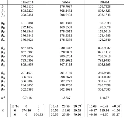
nlmefit, Gibbs sampling, and DRAM. 34
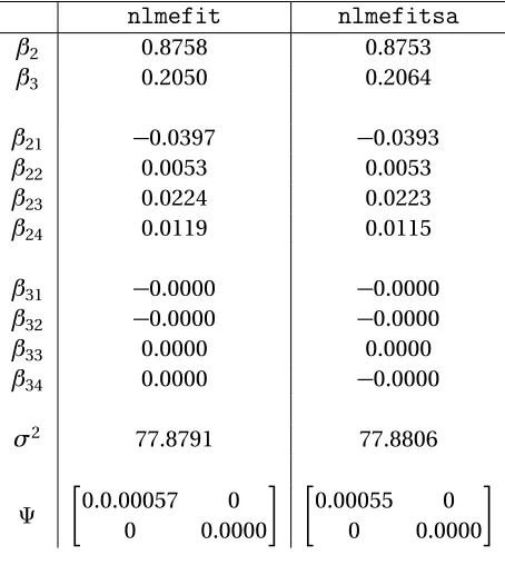
Table 3.2 Estimated parameter values for (3.9) fromnlmefit
andnlmefitsa. . . 37
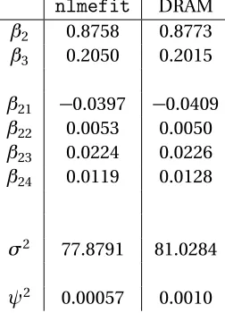
Table 3.3 Estimated parameter values for (3.9) from
nlmefit
andnlmefitsa. . . 38
Table 4.1 Selection scores for (4.6) for all 30 data sets. . . 50
Table 4.2 Selection index sums for the linear mixed-effects model (4.6). . . 50
Table 4.3 Selection scores for the nonlinear mixed-effects orange tree circumference model (4.7). . . 53
Table 4.4 Selection index sums for the nonlinear mixed-effects orange tree circumfer-ence model (4.7). . . 53
Table 4.5 Model selection results for linear model (4.6). The results from PSS-aided model selection are shown along with the results from various other methods as reported in[3]. . . 55
Table 4.6 Model selection results for nonlinear model (4.7) using PSS to aid in model selection. . . 55
Table 5.1 Numerical results from DRAM using the Poisson likelihood (6.2). The reported parameter estimates are the mean chain values. . . 66
Table 5.2 Numerical results from DRAM and DREAM using the Poisson likelihood (6.2) along with the true values used to generate the synthetic data. The reported parameter estimates are the mean chain values. . . 68
Table 6.1 Estimates of background radiation parameters and hyperparameters in the absence of a source obtained from the mean values of the DRAM chains. . . 81
LIST OF FIGURES
Figure 1.1 Flow chart representing the components of predictive estimation in uncer-tainty quantification as described in[37]. . . 2
Figure 2.1 Distributions for parameters (a)q1, (b)q2, and (c)q3constructed using asymp-totic theory, bootstrapping, and DRAM with all four data sets. . . 15 Figure 2.2 Distributions for parameters (a)q1, (b)q2, and (c)q3constructed using
boot-strapping and DRAM with all four data sets. . . 17 Figure 2.3 Residuals for non-linear model (2.2) and linear model (2.5). . . 17 Figure 2.4 Pairwise plots for parameters of (2.2) obtained using DRAM. . . 19 Figure 2.5 Two scenarios involving data collected from multiple experiments modeled
by (2.6). . . 19 Figure 2.6 Three-dimensional plot of data from[27]. . . 22
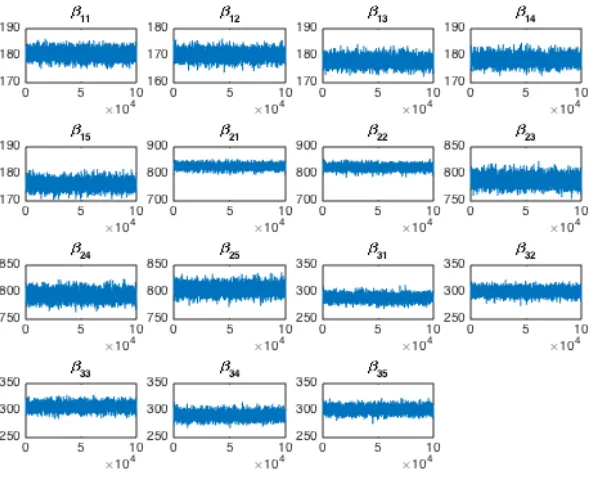
Figure 3.1 Chains generated using DRAM for the effective parameters of the orange tree model (3.7). . . 33 Figure 3.2 Hyperchains generated using DRAM for the components ofβandΨ. . . 35 Figure 3.3 (a) Model fit and (b) residuals for (3.10) using the parameter estimates from
nlmefit. The fit and residuals obtained using
nlmefitsa
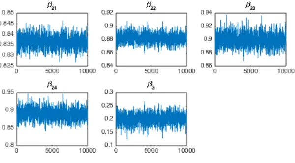
are not pictured because they are visually indistinguishable from those shown here. . . 38 Figure 3.4 Chains generated using DRAM forβ2i=β2+b2iandβ3in model (3.10). . . 39 Figure 3.5 Hyperchains generated using DRAM forβ2andψ2for model (3.10). . . 39 Figure 3.6 (a) The model fit and (b) residuals for (3.10) using the mean DRAM chainvalues as the parameter estimates. . . 40
Figure 4.1 Height measurements in centimeters for 26 boys on nine occasions from[50]. 43 Figure 4.2 Pairwise plots generated by DRAM for the fixed effects of (4.7). . . 51
Figure 5.1 Satellite image of the problem geometry, source location, and stationary detector positions from[39]. . . 58 Figure 5.2 Chains generated by DRAM for source characteristics (a)x, (b)y, and (c)I0. . 66 Figure 5.3 Full DREAM chains for (a)x, (b)y, and (c)I0. Truncated DREAM chains only
including the burned-in portion for (d)x, (e)y, and (f )I0. . . 67 Figure 5.4 Gelman-Rubin R-statistic at each DREAM chain iteration. R-statistic values
below 1.2 suggest that the chain has converged to its stationary distribution. . 67 Figure 5.5 Comparison of marginal pdf’s for source components (a)x, (b)y, and (c)I0
obtained with DRAM and DREAM. . . 68 Figure 5.6 Grid of possible design locations for mobile sensors. . . 72 Figure 5.7 Order in which the sensor locations were employed. The blue x’s indicate the
Figure 5.8 DRAM chains from the final iteration of Algorithm 9 with 25 potential design conditions. . . 75 Figure 5.9 Marginal pdf’s constructed from the DRAM chains of the final iteration of
Algorithm 9 with 25 potential design conditions. . . 75
Figure 6.1 Chains generated using DRAM with Poisson likelihood (6.2) for parameters
rs= (x,y),I0, andBj forj=1, . . . , 10. . . 79 Figure 6.2 Chains generated using DRAM with Poisson likelihood (6.2) for parameters
Bj forj=1, . . . , 10 in the absence of a source. . . 81 Figure 6.3 Chains generated for hyperparametersµandσusing DRAM with Poisson
likelihood (6.2) in the absence of a source. . . 82 Figure 6.4 Chains generated using DRAM with Poisson likelihood (6.2) for parameters
x,y,I0, andBj forj=1, . . . , 10 employing a narrow prior for all background termsBj. . . 82
CHAPTER
1
INTRODUCTION
Uncertainty quantification (UQ) is the science of identifying and reducing sources of uncertainty in
order to make predictions and understand the degree to which these predictions can be trusted. The field of UQ is inherently multidisciplinary, incorporating aspects such as mathematical modeling,
statistics, and numerical analysis. As shown in Figure 1.1, model calibration and parameter selection
are vital aspects of UQ. Model calibration generally serves as an initial step in quantifying uncer-tainties. Parameter selection—typically implemented via sensitivity analysis or active subspace
construction—isolates a subset or subspace of influential and identifiable parameters. This aids
model calibration by reducing the number of parameters to be estimated and ensuring that there exists a unique set of inferred parameters.
1.1
Model Calibration
Model calibration involves optimally inferring parameters to match the model output to a physical
response obtained from measurement data. For the purposes of UQ, we also want to quantify, or possibly update, the uncertainty in these optimal parameter estimates. We can accomplish this either
by constructing parameter distributions or by determining confidence intervals about a parameter
Uncertainty Propagation
Stochastic Spectral Methods Model Calibration
Local Sensitivity Analysis Global Sensitivity Analysis Parameter Selection
Model Discrepancy
Surrogate Models
Sparse Grids Input Representation
Sparse Grids
Figure 1.1: Flow chart representing the components of predictive estimation in uncertainty quan-tification as described in[37].
occur when a large number of experiments are performed. Thus, a frequentist views the concept of
probability as a deterministic value that does not change regardless of experimental data. Similarly,
parameters are also viewed as fixed but unknown values, which are not affected by the collection of additional response data. To estimate these fixed parameter values, we construct estimators
for assigning optimal parameter values based on response data. These estimators are functions
of random variables that map the sample space—that is, the set of all possible observations—to a set of parameter estimates. Hence, the estimators themselves are considered random variables,
each with an associated sampling distribution. Since the parameters are assumed to have a true,
fixed value, parameter uncertainty from a frequentist perspective is simply the uncertainty of the estimator, which is represented by its sampling distribution[37].
The Bayesian perspective defines probability as a quantified measure of the belief that an event
will occur based on available information and prior knowledge[1]. Note that this interpretation of probability is subjective; hence, Bayesian probabilities are not fixed values and can change as more
information is acquired. As another departure from the frequentist framework, Bayesian parameters
are regarded as random variables; their associated distributions characterize the current “state of knowledge" about the parameter value. Hence, the task of Bayesian parameter estimation involves
constructing the parameter probability density function (pdf ), which is termed the “posterior
on observations and prior information, Bayes’ theorem
P(A|B) =P(B|A)P(A) P(B)
for eventsAandB whereP(∗)denotes the probability of an event occurring provides a natural foundation for parameter estimation. Thus, to infer parametersQ= [Q1,Q2, . . . ,Qp]based on obser-vationsν= [ν1,ν2, . . . ,νn], we employ Bayes’ relation
π(q|ν) =R π(ν|q)π0(q) Rpπ(ν|q)π0(q)d q
, (1.1)
whereπ(q|ν)is the posterior parameter pdf,qrepresents realizations ofQ,π0(q)is the prior distri-bution,π(q|ν)is the likelihood function, and the marginal pdf represented by the integral in the denominator is a normalization factor[37]. While (1.1) appears to be a straightforward formula for
obtaining the posterior density, its implementation can be difficult in practice. The normalization
factor in the denominator can rarely be calculated analytically, so numerical methods such as quadrature techniques must instead be applied. This is similarly true for the integral evaluations
required to obtain marginal posterior densities from the joint posteriorπ(q|ν). As an alternative to numerically evaluating theses integrals, we can construct Markov chains whose stationary distribu-tion is the posterior density as is done in Markov Chain Monte Carlo (MCMC) techniques[37]. In
Chapter 2, we construct distributions using both frequentist and Bayesian techniques to explore
parameter uncertainty.
1.2
Sensitivity Analysis
Sensitivity analysis involves quantifying the relative contributions of parameters or inputs to the model output[37]. One important application of sensitivity analysis is parameter selection. Once
insensitive parameters are identified, they can be fixed rather than estimated with minimal impact
on the model response. This is particularly beneficial for models in biology and physics, which often have hundreds of parameters[45]. Reducing the number of parameters, especially in
high-dimensional problems, greatly improves the efficiency—and sometimes the feasibility—of model calibration.
Sensitivity analysis techniques are divided into two categories: local and global. Local
sensi-tivity analysis methods examine how the model response varies when the parameters or inputs are perturbed about a nominal value. Partial derivatives are typically employed to quantify local
sensitivities, but they are often impossible or infeasible to calculate directly. Whereas adjoint
techniques for obtaining local sensitivities include finite difference approximations, solutions to
sensitivity equations, and automatic differentiation[37]. Whereas the majority of sensitivity analysis literature focuses on local techniques, such methods can be problematic for determining the global
effect of parameters, especially in highly nonlinear problems[33, 37]. When the sensitivity over the
entire parameter space is of interest, global techniques are advantageous.
Global sensitivity techniques ascertain the relative contributions of parameter uncertainty to
the uncertainty in the model output over the entire possible range of parameter values. Such global
sensitivities depend solely on the model and response and are not affected by experimental data[37]. Variance-based global sensitivity methods, such as the calculation of Sobol’ indices, apportion the
variance of the output Var(y)to the variance of the parameters. To do this, we rank the parameters q= [q1,q2, . . . ,qp]based on the amount of variance that is removed from the output when a particular parameter is fixed. Ideally, we would fix the parameters, setting them equal to nominal valuesqi∗, and calculate Var(Y|qi=qi∗)for each parameterqi, but these values ofqi∗are generally unknown. We instead take the average of the variance over all possible values ofqi, namelyE Var(y|qi)
[34]. Although some would recommend using variance-based methods whenever possible[33], these
sensitivity methods are computationally demanding, which often makes them infeasible for complex
and high-dimensional problems. In such cases, Morris screening provides an appealing alternative. The idea of Morris screening is to average local sensitivity information, essentially finite difference
approximations of partial derivatives, taken throughout the parameter space to obtain a more global measure of sensitivity. Unlike variance-based methods, Morris screening only provides a
relative ranking of parameter significance; it does not give a measure of how much more significant
a higher-ranking parameter is[37]. In spite of providing less information, Morris screening remains a popular choice for global sensitivity analysis due to its computational efficiency.
1.3
Uncertainty Quantification for Mixed-Effects Models
Mixed-effects models are commonly used to statistically model phenomena that include attributes
associated with a population or general underlying mechanism as well as effects specific to
individ-uals or components of the general mechanism. This can include individual effects associated with data from multiple experiments. When appropriate, the incorporation of mixed-effects can reduce
model discrepancy and provide a means for quantifying individual variation of parameter values
within populations.
Despite the advantages of using this framework, uncertainty quantification for mixed-effects
models is particularly challenging since UQ techniques established for traditional modeling
gen-erally prove incompatible or ineffective with this type of model. In this dissertation, we focus on parameter estimation and sensitivity analysis methods for mixed-effects models. In Chapter 3,
estimation and introduce a modified version of the Delayed Rejection Adaptive Metropolis (DRAM)
algorithm for mixed-effects models. Current frequentist methods for mixed-effects parameter esti-mation, which involve on maximum likelihood estiesti-mation, are available in MATLAB via the Statistics
Toolbox. The standard Bayesian technique for mixed-effects models is Gibbs sampling, which is also
utilizing for some parameter updates in our modified DRAM algorithm. In Chapter 4, we demon-strate the problems with applying traditional sensitivity analysis techniques to mixed-effects models
and propose an efficient method for mixed-effects parameter selection that is effective for both
linear and nonlinear problems. While traditional sensitivity analysis techniques fail to distinguish between the global parameters and the parameters quantifying individual variations, our parameter
subset selection algorithm, based on standard errors, accurately ranks both types of parameters for
mixed-effects models.
1.4
Applications
Mixed-effects models have applications in many areas of science and engineering. We specifically ex-plore nuclear engineering applications, focusing on problems that are of interest to theConsortium
forAdvancedSimulation ofLight-water Reactors (CASL) and to theConsortium forNonproliferation
EnablingCapabilities (CNEC).
1.4.1 CASL Applications
CASL was founded with the purpose of improving modeling and simulation for the light-water
reactor (LWR). Unlike heavy water reactors used in Canada and India, light-water nuclear reactors
employ ordinary water as a coolant and neutron moderator[37]. With the aim of modeling this reac-tor type, CASL created theVirtualEnvironment forReactorApplications (VERA). This environment
includes capabilities for thermal-hydraulics analysis, which is crucial for modeling the behavior of
the coolant. The coolant in the LWR is present in both liquid and vapor form; hence, we require a two-phase model.
Letαgandαf represent the volume fractions for the gas and fluid phases. We respectively denote the densities and velocities of the gas and fluid phases asρg,ρf andνg,νf. Let the internal energies of gas and fluid be denoted byegandef . Now, using conservation of mass, momentum, and energy, we can model the fluid phase relations as
∂
αfρf ∂ νf
∂t +αfρfνf · ∇νf +∇ ·σ R
f +αf∇ ·σ+αf∇ρf =−FR−F +Γ(νf −νg)/2+αfρfg,
and
∂
∂t(αfρfef) +∇ ·(αfρfefνf +T h) = (Tg−Tf)H+Tf∆f −Tg(H−αg∇ ·h) +h· ∇T −Γ[ef +Tf(s∗−sf)]
−pf
∂ α
f
∂t +∇ ·(αfνf) +
Γ
ρf
,
whereTf is the fluid temperature,sf is the fluid entropy density,pf is the continuous phase pressure, σis the viscous transport coefficient, andκ,ζ, andγare positive transport coefficients[37]. The coupled relations for the gas phase are analogous. In addition to these equations, numerous closure
relations, such as the Dittus-Boleter equation, are needed to model the coolant. In Chapter 2, we
introduce a parameterized version of the phenomenological Dittus-Boelter equation. We then construct pdf’s for the parameters and illustrate the need for model modifications, including the
incorporation of mixed-effects.
1.4.2 CNEC Applications
CNEC, funded by a grant from the National Nuclear Security Administration (NNSA), is comprised of seven universities (North Carolina State University, Georgia Institute of Technology, Kansas State
University, North Carolina A&T State University, Purdue University, University of Illinois at
Urbana-Champaign, and University of Michigan) and three national laboratories (Los Alamos, Oak Ridge, and Pacific Northwest National Laboratories). This consortium supports research in the detection
and characterization of special nuclear materials (SNM) as well as in the detection of facilities
producing SNM. CNEC members also investigate feasible replacements for industrial radiation sources as a means to prevent their misappropriation such as being used to build dirty bombs.
In accordance with the goals of CNEC, we investigate radiation detection in an urban setting in
Chapters 5 and 6. Given responses from radiation detectors, we wish to determine the radiation source intensity and location. In Chapter 5, we solve this inverse problem for stationary detectors
using a simplified radiation transport model. However, this model does not account for variation in background radiation among the detector locations. We introduce a mixed-effects model in Chapter
6 to account for the varying background term. In addition to stationary radiation sensors, we also
1.5
Dissertation Contributions and Organization
In this dissertation, we introduce two new UQ techniques for mixed-effects models: a mixed-effects
version of the DRAM algorithm and a parameter subset selection (PSS) algorithm. The DRAM algorithm for mixed-effects models provides a new method of Bayesian parameter estimation,
and the PSS algorithm aids mixed-effects model selection when traditional sensitivity analysis
techniques are ineffective. Moreover, we employ mixed-effects modeling for a variety of nuclear engineering problems, including radiation detection in an urban setting. The organization of this
dissertation, based on the contents of the chapters, is detailed below.
• Chapter 2
We introduce a parameterized version of the Dittus-Boelter equation, which serves as a
mo-tivating example for the use of mixed-effects modeling. As mentioned in Section 1.4.1, the
Dittus-Boelter equation is important to the CASL initiative because it serves as one of the closure relations in the LWR coolant model. We construct parameter pdf’s for the
parame-terized Dittus-Boelter equation using three methods: asymptotic analysis, bootstrapping,
and DRAM. Also, we provide a plot of experimental data that suggests that the Dittus-Boelter model parameters are inconsistent among data sets, indicating that use of mixed-effects
modeling is advisable.
• Chapter 3
We formally introduce the structure of mixed-effects models and highlight the parameter estimation techniques for such models. Using functions from the MATLAB Statistics
Tool-box, we perform frequentist parameter estimation, via maximum likelihood estimation, for
both linear and nonlinear mixed-effects models. For Bayesian parameter estimation, Gibbs sampling is the current standard, but some efforts have been made to expand the DRAM
algorithm to mixed-effects models. In particular, the MATLAB MCMC Toolbox DRAM code
contains an option for estimating mixed-effects parameters with independent random effects. We expand upon this and introduce a novel version of the DRAM algorithm for mixed-effects
models with non-diagonal random effects covariance matrices.
• Chapter 4
When performing sensitivity analysis for mixed-effects models, traditional techniques are generally ineffective, failing to distinguish between the global and local effects. In the
mixed-effects literature, the isolation of sensitive parameters is instead achieved with model selection
via information criteria. However, this process can be computationally prohibitive, especially for high-dimensional problems. Alternatives to this type of model selection have been
pro-posed, but most of these cannot be applied to nonlinear mixed-effects models. To remedy
models, which is applicable to both linear and nonlinear problems, and use it to reduce the
computational cost of model selection with information criteria.
• Chapter 5
Here we introduce the problem of radiation source localization. We first consider the case
of stationary radiation detectors. To simulate a radiation source in downtown Washington
D.C., we use a simplified photon transport equation to generate the detector responses. Using this data, we solve the inverse problem to determine the intensity and location of the source.
In this chapter, we do not employ mixed-effects for our detector response model; we simply
employ the photon transport equation used to generate the data as our model. We perform parameter estimation via DRAM and the Differential Evolution Adaptive Metropolis (DREAM)
algorithm. We also consider source localization with mobile sensors. We propose the use
of mutual information to guide the movement of the radiation detectors. In particular, we provide an algorithm that determines the optimal measurement location from a set of possible
design conditions using mutual information.
• Chapter 6
The simplified photon transport model from Chapter 5 does not account for varying back-ground radiation among the detector locations. Thus, we incorporate mixed-effects to allow
for individual background We apply the mixed-effects DRAM algorithm form Chapter 3 to
estimate the source location and intensity along with the individual background parameters for each source. We initially used flat priors for all of the parameters and discovered that the
parameter set is not mutually identifiable. We use the term “flat prior" rather than "uniform
prior" throughout this disseration because the employed prior distributions may not integrate to unity and may, in fact, be improper; e.g. for parameters with the admissible space[0,∞). We then calibrated the background radiation parameters in the absence of a source to obtain
better prior information for the background terms. Use of this narrow prior distributions allowed us to simultaneously estimate all of the model parameters without experiencing
CHAPTER
2
STATISTICAL INFERENCE FOR THE
DITTUS-BOELTER EQUATION
The Dittus-Boelter equation for heated liquids is
N u=0.023R e0.8P r0.4, (2.1)
whereN uis the Nusselt number,R e is the Reynolds number, andP r is the Prandtl number with P r having an exponent of 0.3 for cooling liquids. This empirical relation is frequently used for
approximate calculations in engineering. Pinpointing the origin of the equation in its final form is
somewhat challenging with many authors referencing papers that do not contain the equation at all
[47]. The most likely true origin is McAdams’s 1942 textbook[26]with the author slightly modifying the values of the coefficient and exponents compared to earlier versions of the equation.
The Dittus-Boelter equation was first developed to describe heat transfer in the smooth pipes of automobiles, but it is currently employed by CASL to describe heat transfer in light-water nuclear
reactors[28]. Currently, CASL utilizes the thermal hydraulic code CTF—originally called COBRA-TF
before its rebranding—as a component of its virtual reactor (VERA)[32]. CTF uses the Dittus-Boelter equation to model heat transfer from the solid wall to fluids of certain regimes in the reactor pipes.
In particular, the Dittus-Boelter equation is used for fluids that are categorized as single-phase
correlations, which are modified versions of the Dittus-Boelter equation[28].
The nominal values of 0.023, 0.8, and 0.4 from (2.1) were obtained via fitting the data by hand for a specific regime. Since the Dittus-Boelter has taken various forms[47]due to varying calibration
regimes and the use of rudimentary parameter estimation methods, we utilize a parameterized
version to obtain more accurate coefficient and exponent values via parameter estimation. Thus, for modeling the behavior of heated liquids, we consider the statistical model
N u(q,R e,P r) =q1R eq2P rq3+", (2.2)
whereN u is the Nusselt number,R e is the Reynolds number,P r is the Prandtl number, and"is the measurement error. We assume that the measurement errors are independent and identically
distributed (iid); in particular,"∼ N(0,σ2). Note that (2.2) is a parameterized version of the Dittus-Boelter equation (2.1).
2.1
Parameter Probability Density Functions
Whereas we seek to calibrate the model (2.2) via parameter estimation, we also aim to quantify the
uncertainty of these parameter estimates. We do this by constructing parameter probability density
functions (pdf’s). To implement parameter estimation and uncertainty quantification, we employed experimental data sets from[27], namely groups of ordered triples containing recorded
measure-ments of the Reynolds, Prandtl, and Nusselt numbers. We utilized four such groups corresponding
to four different steam-heated liquids: water, gas oil, straw oil, and light motor oil. Given the four data sets—which respectively contained 12, 13, 22, and 9 data points—we constructed pdf’s for
the parameter setq= [q1,q2,q3]using three methods: asymptotic analysis, bootstrapping, and the
Delayed Rejection Adaptive Metropolis (DRAM) algorithm.
2.1.1 Asymptotic Analysis
As explained in Chapter 1, the frequentist approach to quantifying parameter uncertainty involves examining the sampling distribution, which characterizes the uncertainty in the performance of
the estimator. For asymptotic analysis, we consider the behavior of the sampling distribution as n→ ∞wherenis the number of data points. Here, we examine the asymptotic behavior of the sampling distribution associated with the nonlinear ordinary least squares (OLS) estimator.
Let a general nonlinear statistical model be represented by
Υ=f(q0) +"
repre-sents the true but unknown frequentist parameter vector, and"= ["1,"2, . . . ,"n]T is the vector of measurement errors. As with the Dittus-Boelter model (2.2), we assume that the errors are iid and normally distributed with a mean of zero and fixed but unknown variance, which we denote here as σ2
0. The nonlinear OLS estimator and estimate are defined as
qO LS=argmin q∈Q
n
X
i=1
Υi−fi(q)
2
, (2.3)
ˆ
qO LS =argmin q∈Q
n
X
i=1
υi−fi(q)
2
,
whereQis the space associated with the estimatorqO LS,Qis the admissible parameter space, and
υ= [υ1,υ2, . . . ,υn]is the vector of experimental observations. Hence, the parameter estimate ˆqO LS is obtained from minimizing the cost function
J(q) = n
X
i=1
υi−fi(q)
2
(2.4)
subject toq ∈Q. For nonlinear problems, (2.4) generally does not have an analytic solution, so
we instead minimize the cost function numerically. In this dissertation, we employ the MATLAB function
fminsearch
to obtain nonlinear OLS estimates. Since the error variance is also fixed butunknown, we also construct an OLS estimator and estimate
σ2
O LS = 1 n−pR
TR
ˆ σ2
O LS = 1 n−pRˆ
TRˆ
for the error variance wherepis the number of parameters. Here,R=Υ−f(qO LS)andR=υ−f(qˆO LS) aren×1 column vectors respectively corresponding to the residual estimator and estimate.
With the assumption that"i ∼ N(0,σ20), the nonlinear OLS estimator is consistent—that is, for a sufficiently large sample size,E(qO LS) =q0—as well as asymptotically normal[36, 37, 38]. In particular, given a large number of data points, the sampling distribution can be accurately
approximated asqO LS∼ N(q0, ˆVO LS), where ˆVO LS is the OLS estimate of covariance given by
ˆ
VO LS=σˆ2O LS[χT(qˆO LS)χ(qˆO LS)]−1.
Hereσ2O LS is the OLS estimate of error variance andχ(q)represents the sensitivity matrix
χi k(qˆO LS) =
evaluated at the OLS estimate ˆqO LS. Hence, when we use asymptotic theory to construct the sampling distribution, we assume that our number of data points is sufficiently large to enter the asymptotic regime and simply employ a multivariate Gaussian distribution utilizing the OLS estimates ˆqO LS and ˆVO LS as the mean and covariance, respectively.
2.1.2 Bootstrapping
Whereas asymptotic analysis is computationally efficient, there are many conditions required for
its accurate characterization of the sampling distribution beyond a rough approximation. In the previous section, we assumed that we have a “large enough" sample size to apply asymptotic
properties. The number of data points that constitute a sufficiently large sample is often ambiguous, but it is clear that asymptotic theory will not perform well for small data sets. Moreover, many of the
results described previously for the nonlinear OLS estimator and its asymptotic properties were
derived using a linear Taylor series expansion along with the assumption of local linearity to exploit existing theory for the linear OLS estimator[37, 36]. For highly nonlinear problems, the assumption
of local linearity is no longer valid, and the results for the previous section cannot be applied.
Bootstrapping provides an alternative method to construct sampling distributions associated with frequentist estimators. Bootstrapping outperforms asymptotic theory for small sample sizes,
and we can relax the assumption that the errors are iid and normally distributed to requiring that
they are simply iid. Moreover, bootstrapping techniques are not rooted in linear theory, so we no longer require the assumption of local linearity and may freely employ such methods for highly
nonlinear problems[7].
When we apply bootstrapping from a frequentist perspective, we seek to determine the uncer-tainty of an estimator by constructing its sampling distribution. We again consider the nonlinear
OLS estimator, and we estimate the parameters based on (2.3) usingn data points. Ideally, we
would get a sense of the distribution associated with the OLS parameter estimates by repeatedly resampling to obtain new data points and applying (2.3) to recalculate the parameter estimates.
In particular, we would obtain Monte Carlo approximations to the parameter distributions if the
number of resampling iterations was large. However, resampling to obtain new data points is often either impossible or impractical. The idea of bootstrapping is to use thendata points in place of
the larger population and sample from the original data points with replacement. As detailed in[7],
bootstrapping follows these general steps:
1. Sample with replacement from the originalndata points; this newly sampled set is called the “bootstrap sample."
2. Compute estimate(s) using the desired estimator with the bootstrap sample.
For large enoughM, we are essentially constructing a Monte Carlo approximation of the estimator
sampling distribution, but we are drawing from an empirical distribution, which assigns a prob-ability of 1/nto each of the originally-collected data points, in place of the unknown population distribution.
With the idea of bootstrapping in place, it may seem reasonable to approach the problem of constructing parameter pdf’s for the Dittus-Boelter model (2.2) by obtaining a large number of
bootstrap samples from the collected ordered triples[R ei,P ri,N ui], estimating the the parameters q1,q2, andq3 for each bootstrap sample, and using the set of the estimates to obtain a Monte Carlo approximation to the parameter distributions. However, this approach can be theoretically
problematic; it treats the design conditions—in this case,R e andP r—as random rather than fixed,
which is inappropriate for experiments necessitating measurements under specific designs[12]. To treat the design conditions as fixed, we utilize the bootstrapping method described in Algorithm 1.
This method treats the originally-collected data as fixed and instead resamples the residuals of the
Algorithm 1Construction of Parameter pdf’s via Bootstrapping[16]
1. Set ˆqO LS equal to the ordinary least square estimate of the parameter vector.
2. Form=0, 1, . . . ,M−1, whereM is the number of bootstrapping samples, Forj=0, 1, . . . ,n−1, wherenis the number of data points,
(a) Construct set of standardized residuals{rj}nj=0as
rj =
v
t n
n−p
yj −f(x, ˆqO LS)
,
wherepis the number of parameters,f is the model function, andxis the vector of
design conditions.
(b) Sample from{rj}nj=0with replacement to generate a bootstrap sample ofn standardized residuals
˜
r0m, ˜r1m, . . . , ˜rnm−1 .
(c) Generate synthetic datayjm=f(x, ˆqO LS) +r˜jm.
(d) Using the synthetic data, calculate the ordinary least squares estimate to obtain ˜qm.
3. This generates bootstrap samplesq˜0, ˜q1, . . . , ˜qM−1 .
2.1.3 Delayed Rejection Adaptive Metropolis (DRAM)
Recall from Chapter 1 that Bayesian parameter estimation entails constructing posterior densities, which represent the "state of knowledge" about the parameter. Since the constructed posterior
densities inherently characterize parameter uncertainty, this approach to parameter estimation is
natural for the goals of UQ. Here, we employ the DRAM algorithm for Bayesian parameter estimation and, hence, for building parameter pdf’s.
The DRAM algorithm[15, 37]is a modified version of the Metropolis-Hastings algorithm, a
Markov Chain Monte Carlo (MCMC) technique used to randomly sample from probability distri-butions. In the case of Bayesian inference, the Metropolis-Hastings algorithm is used to sample
from the posterior parameter densities. The DRAM algorithm—detailed in Algorithms 2 and 3 for problems employing a normal likelihood function—adds two additional steps, which correspond
to adaptation and delayed rejection. The adaptive step allows for the geometry of the proposal
de-layed rejection step improves the mixing of the chains. In order to achieve good exploration of the
parameter space via the proposal distributionN(θk−1,Vk−1), it is important that the covariance matrix reflect the geometry of the parameter space. The incorporation of the adaptation step allows
for a poor initial estimate of the covariance to be corrected, enabling a more efficient exploration of
the chains.
To implement DRAM, we used OLS estimates as the starting values ofq1,q2, andq3. We bounded
each of the parameters with a lower limit of zero and an upper limit of two times the nominal
values from (2.1); this is standard practice in the nuclear engineering literature when computing uncertainties. We used the least squares estimate of variance ˆσ2O LS=186.0443 for the initial value of the error variance. For design parameters, we chosens=1,σ2s =σˆO LS2 ,sp=2.382/p, andk0=100. With this setup, we implemented the DRAM code from the MATLAB MCMC Toolbox available for download at
http://helios.fmi.fi/∼lainema/mcmc/. After a burn-in period of 10
4iterations,we reran the code for 105iterations starting with the results from the previous run. We obtained the
DRAM estimate error variance by taking the mean of the resulting error variance chain.
2.2
Results
Figure 2.1 shows the parameter pdf’s obtained using asymptotic analysis, bootstrapping, and DRAM with 56 points pooled from the four data sets. The resulting distributions are similar for all three
methods, but those generated via bootstrapping and DRAM are nearly visually indistinguishable.
Since we are using a flat prior and a normal likelihood function with DRAM, the Bayesian technique should only agree with a frequentist method if the problem is linear or if the parameter distributions
are Gaussian. However, the Dittus-Boelter model (2.2) is clearly nonlinear, and Figure 2.2 also shows
0 0.002 0.004 0.006 0.008 0.01 0 100 200 300 400 500 q1 DRAM Bootstrap Asymptotic (a)
0.9 0.95 1 1.05 1.1 1.15 0 5 10 15 20 q2 DRAM Bootstrap Asymptotic (b)
0.35 0.4 0.45 0.5
0 5 10 15 20 25 30 35 q3 DRAM Bootstrap Asymptotic (c)
that theq1parameter distribution is slightly skewed and, therefore, non-Gaussian. This suggests
that the model might exhibit linear behavior in the observed region.
To examine this possibility, we consider—as an alternative to (2.2)—the statistical model
N u(q,R e,P r) =f(qn o m,R e,P r) +D f(qn o m,R e,P r)(q−qn o m) +" (2.5)
based on linearization about the nominal parameter valuesqn o m= [0.023, 0.8, 0.4], where
f(q,R e,P r) =q1R eq2P rq3
and
D f(q,R e,P r) =
∂f ∂q1
q,R e,P r , ∂f
∂q2
q,R e,P r , ∂f
∂q3
q,R e,P r
.
Implementing the DRAM algorithm for this model, we used the least squares parameter estimates ˆ
qO LS = [−0.4457, 2.3509, 1.6019]as the starting values of the parameters, and we used the least squares estimate of variance for the initial value of the error variance. No bounds were placed on the parameters. After a burn-in period of 104iterations, we reran the DRAM code for 105iterations
starting with the results from the previous run. Using the mean values of the estimated parameter
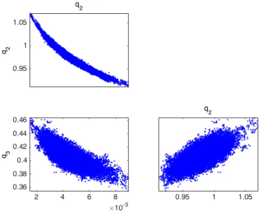
distributions, we calculated the residuals for the nonlinear model (2.2) and the linear model (2.5). A plot comparing the residuals for both models is given in Figure 2.3. The residuals are very similar
in pattern and size, suggesting that the two models provide similar fits. Hence, it is likely that the
model behavior is approximately linear in the observed region, which explains the agreement of the parameter distributions obtained from bootstrapping and DRAM.
Table 2.1 gives a comparison of the mean values of the three constructed distributions and the
nominal parameter values. While the means of all three distributions agree, these values are notably different for parametersq1andq2. Since we also see a reduction in our estimation of uncertainty,
this suggests that the parameter estimates for all three methods are an improvement of the nominal
values used in (2.1). This reduction in uncertainty is characterized by the 95% confidence intervals for the frequentist methods and the 95% credible intervals for DRAM given in Table 2.2. Note that
the intervals derived from the constructed pdf’s are much narrower than the nominal interval of
uncertainty.
2.3
Model Improvements
Whereas we were able to successfully construct pdf’s for the parameters of (2.2) with the results suggesting estimates that are reasonably close to the nominal values, closer examination reveals the
0 0.002 0.004 0.006 0.008 0.01 0 100 200 300 400 500 q1 DRAM Bootstrap (a)
0.9 0.95 1 1.05 1.1 1.15 0 5 10 15 20 q2 DRAM Bootstrap (b)
0.35 0.4 0.45 0.5
0 5 10 15 20 25 30 35 q3 DRAM Bootstrap (c)
Figure 2.2: Distributions for parameters (a)q1, (b)q2, and (c)q3constructed using bootstrapping and DRAM with all four data sets.
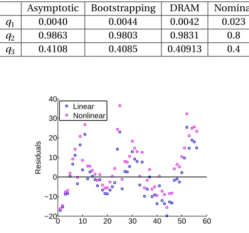
Table 2.1: Comparison of the nominal values to the means of the parameter pdf’s constructed via asymptotic analysis, bootstrapping, and DRAM.
Asymptotic Bootstrapping DRAM Nominal
q1 0.0040 0.0044 0.0042 0.023
q2 0.9863 0.9803 0.9831 0.8
q3 0.4108 0.4085 0.40913 0.4
0 10 20 30 40 50 60
−20 −10 0 10 20 30 40 Residuals Linear Nonlinear
Figure 2.3: Residuals for non-linear model (2.2) and linear model (2.5).
problems. Figure 2.4 shows thatq1andq2have a nearly one-to-one relationship. Hence, if we fix one of the parameters to an arbitrary value, we could find a corresponding value for the other parameter
that optimally fits the model to the data. This means that the parameter setq = [q1,q2,q3]is not
Table 2.2: The 95 % confidence intervals for asymptotic theory and bootstrapping as well as the 95% credible intervals for DRAM compared to the nominal uncertainty.
Asymptotic Intervals Bootstrapping Intervals DRAM Intervals Nominal Uncertainty q1 [0.0021, 0.0059] [0.0023, 0.0065] [0.0025, 0.0064] [0, 0.046] q2 [0.9436, 1.0291] [0.9377, 1.0228] [0.94401.0262] [0, 1.6] q3 [0.3857, 0.4359] [0.3836, 0.4335] [0.3853, 0.4353] [0, 0.8]
We can resolve this issue by fixing eitherq1orq2in the model (2.2) and estimating the remaining
two parameters.
In addition to identifiability problems, we have the issue of incompatible parameters. To
under-stand incompatible parameters, we present in Figure 2.5 a comparison of two scenarios in which
data is modeled by a parameterized version of the McAdams relation[46]
F =ξ1R eξ2+" (2.6)
whereF is the friction factor,R eis the Reynolds number,ξ1andξ2are parameters, and"represents measurement error. In one scenario, the data points from 5 experiments are aligned in such a way
that a single model curve—and, hence, a single set of optimal parameters—provides a reasonable
fit for all data sets. However, this is not true of the second scenario. While the shape of the curves are similar for all of the experimental data sets, suggesting the same underlying physics, there is
not one set of parameter values that will optimally fit all of the data sets. As shown in Figure 2.6, a
similar situation arises with the data from[27]for the Dittus-Boelter problem. To remedy this type of situation, we need to account for parameter variability among the individual data sets and allow for
individual fits. Ideally, we would also like to quantify “nominal" parameter values that adequately
represent all data sets. In Chapter 3, we introduce mixed-effect models as a way to account for variability within a population of parameters. We also present techniques for estimating parameters
of mixed-effects models and employ them for an improved version of (2.2), which remedies the
Figure 2.4: Pairwise plots for parameters of (2.2) obtained using DRAM.
●
● ● ●
● ● ● ● ●
●
●
0e+00 1e+05 2e+05 3e+05 4e+05 5e+05
0.015
0.020
0.025
0.030
Reynolds number
F
●Exp. 1 Exp. 2 Exp. 3 Exp. 4 Exp. 5
Desirable Situation
●
● ● ●
● ● ● ● ●
●
●
0e+00 1e+05 2e+05 3e+05 4e+05 5e+05
0.01
0.02
0.03
0.04
0.05
Reynolds number
F
●Exp. 1 Exp. 2 Exp. 3 Exp. 4 Exp. 5
Reality
nominal model
Algorithm 2Delayed Rejection Adaptive Metropolis with a Normal Likelihood Function and a Flat Prior Distribution[15, 37]
1. Set design parametersns,σ2s,spandk0and the number of chain iteratesM. Herensandσ2sare employed to update the error variance. The design parameterspdepends on the dimension of the problem; we usesp=2.382/p. Also,k0denotes the number of iterations between updates of the covariance matrix.
2. Determineq0=arg min
q
Pn
i=1[vi−fi(q)]2. 3. SetSSq0=
Pn
i=1[νi−fi(q0)]2.
4. Compute initial variance estimates02=SSn−qp0, wherenis the number of data points andp is the number of parameters.
5. Construct initial variance estimateV0=s02
χT(q0)χ(q0)−1
and setR0=chol(V0), where the
sensitivity matrix has componentsχi j=
∂fi(q0) ∂qj
.
6. Fork=1, ...,M
(a) Samplezk∼ N(0,I).
(b) Construct candidateq∗=qk−1+RT k−1zk.
Note that this is equivalent to samplingq∗∼ N(qk−1,V
k−1). (c) Sampleuα∼ U(0, 1).
(d) ComputeSSq∗=
Pn
i=1[νi−fi(q∗)]2. (e) Compute
α(q∗|qk−1) =min
1,e−
SSq∗−SSq k−1
/2s2
k−1
.
(f ) Ifuα< α,
Setqk=q∗,SSqk=SSq∗.
else
Enter Delayed Rejection Algorithm 3.
endif
(g) Updatesk2∼Inv-gamma(av a l,bv a l), where av a l =0.5(ns+n),bv a l =0.5(nsσ2s+SSqk).
(h) If mod(k,k0) =1,
UpdateVk=spcov(q0,q1, ...,qk)andRk=chol(Vk). else
Vk=Vk−1,Rk=Rk−1.
Algorithm 3Delayed Rejection Component of DRAM with a Normal Likelihood Function[15, 37]
1. Set the design parameterγ2<1. We setγ2=15. 2. Samplezk∼ N(0,I).
3. Construct second-stage candidateq∗2=qk−1+γ
2RkT−1zk. Note that this is equivalent to samplingq∗2∼ N(qk−1,γ22Vk−1). 4. Sampleuα2∼ U(0, 1).
5. ComputeSSq∗2=
Pn
i=1[νi−fi(q∗2)]2. 6. Compute
α2(q∗2|qk−1,q∗) =min
1,π(qπk(q−1∗2|v|ν))JJ(q(q∗∗||qqk∗−21)[)[11−α−α(q(q∗|∗q|q∗2k)]−1)]
,
whereπis the normal likelihood function andJ is the proposal, or jumping, distribution in (6a-b) of Algorithm 2. Specifically,
J(qa|qb) =p 1
(2π)p|V|exp
−1 2
(qa−qb)V−1(qa−qb)T
.
7. Ifuα2< α2,
Setqk =q∗2,SSqk=SSq∗2.
else
Setqk =qk−1,SSqk=SSqk−1.
4
#104 3
Re
2 1 0 0 200 400
Pr
600 0 50 100 150 200 250 300 350 400 450
800
Nu
data set 1 data set 2 data set 3 data set 4
CHAPTER
3
PARAMETER ESTIMATION TECHNIQUES
FOR MIXED-EFFECTS MODELS
Varying responses within a population can be described by a mixed-effects model. Such a model
includes fixed, population-wide effects as well as random effects, which incorporate individual
variation. The statistical mixed-effects model takes the form of
yi j=f(xi j;β,bi) +"i j (3.1)
where, for each individuali,yi jis thejth observation,xi jis the jth vector of independent variables, βis the vector of fixed-effect parameters,bidenotes the vector of random effects, and"i j is the measurement error. It is assumed that
bi∼ N(0,Ψ) (3.2)
"i j∼ N(0,σ2),
whereΨis the covariance matrix of the random effects andσ2is the variance of the measurement errors. Note that the covariance matrixΨis diagonal if the random effects for each individual are
parametersβi=β+bifor each individuali are estimated in place of the random effects.
3.1
Current Parameter Estimation Techniques
3.1.1 Frequentist Methods
Parameter estimation in the frequentist framework involves constructing an estimator, which assigns optimal parameter values based on the observed data. Recall from Chapter 1 that the parameters in
frequentist inference are considered fixed but unknown and that the data are considered realizations
of random variables. In Chapter 2, we utilized the Ordinary Least Squares (OLS) estimator to obtain optimal parameter values. Here we employ maximum likelihood estimation.
To define a maximum likelihood estimator, we first must define a likelihood function. LetfΥ(ν;q)
be a joint probability density function whereq ∈Qis an unknown vector of parameters in the
admissible parameter spaceQ,Υ = [Υ1, . . . ,Υn]is the associated random vector, andν= [ν1, . . . ,νn] are realizations ofΥ. Then, the likelihood functionL:Q→[0,∞), as defined by[37], is given by
L(q) =L(q|ν) =fΥ(ν;q).
We note that the likelihood is a function of the parameters as compared to the sampling distribution,
which is a function of the data. Using this likelihood function with the assumption that the samples νi are iid, we obtain maximum likelihood estimate
ˆ
qM L E =argmax q∈Q
n
Y
i=1
fΥ(νi;q)
as in[37].
Let a general linear mixed-effects model withpF fixed effects andpR random effects be given by
y =Xβ+Z b+" (3.3)
wherey is then×1 response vector,X is then×pF design matrix for the fixed effects,βis thepF×1 vector of fixed effects,Z is then×pR design matrix for the random effects,bis thepR×1 vector of random effects, and"is the vector of measurement errors. We assume that
b∼ N(0,Ψ) =N(0,σ2D(θ)), "∼ N(0,σ2In)
as fixed but unknown parametersβ,σ2, andθ. We have realizationsy for the corresponding vector of random variablesY in the form of data, but the random effects denoted byb are unobserved. Therefore, we must eliminate the dependence onbto obtain a true frequentist likelihood function
L(β,b,σ2,θ|y), which depends only on fixed but unknown parameters and observed random variables.
We now derive the likelihood function as detailed in[21, 30]. Since the random effectsbi for each groupi=1, . . . ,M are independent, it follows that
L(β,σ2,θ|y) = M
Y
i=1
p(yi|β,σ2,θ) = M
Y
i=1 Z
p(yi|β,bi,σ2,θ)p(bi|σ2,θ)|d bi. (3.4)
Note that the probability density functionp(y|β,b,σ2,θ)is a multivariate normal distribution. In particular, we note that
y|β,b,σ2,θ∼ N(Xβ+Z b,σ2In). Thus, we have
p(y|β,b,σ2,θ) = 1
(2πσ2)n/2exp − M P
i=1
kyi−Xiβ−Z bik2 2σ2 = 1
(2πσ2)n/2exp
−ky −Xβ−Z bk2 2σ2
.
Recall thatbi∼N(0,Ψ), so
p(b|θ,σ2) = 1
(2π)pR/2|Ψ|1/2exp
−1 2b
TΨ−1b= 1
(2πσ2)pR/2|D(θ)|1/2exp
− 1 2σ2b
T(D(θ))−1b.
Thus, we have
L(β,σ2,θ|y) =|det[∆(θ)]| (2πσ2)n/2
Z
exp− ky −Xβ−Z bk2+k∆(θ)bk2
/2σ2
(2πσ2)pR/2 d b (3.5)
where ∆(θ)is any matrix such thatD(θ)−1 =∆(θ)T∆(θ). One possibility for∆(θ)is to use the Cholesky factorization ofD(θ)−1. Note that evaluating the integral in (3.5) will still leave occurrences ofb in the right hand side. To eliminate the dependence onb, we find the conditional modes of the
random effects given the data. We first let
r2(β,b,θ) =bT∆(θ)T∆(θ)b+ (y −Xβ−Z b)T(y−Xβ−Z b).
vectorbsatisfy
∂r2(β,b,θ) ∂b
b∗
=0
for givenβandθ. Now, by evaluating the integral in (3.5) and substituting in the vector of conditional modesb∗, we obtain the likelihood function
L(β,σ2,θ|y) =|det[∆(θ)]| (2πσ2)n/2 exp
§
− 1 2σ2r
2(β,b∗(β,θ),θ)ª 1
|∆T∆+ZTZ|1/2. (3.6)
While (3.6) represents a valid likelihood function, a profiled likelihood, which reformulates (3.6) to exclusively be parameterized byθ, is generally used in practice for numerical optimization[21]. This is achieved by deriving formulas for the conditional estimatesβ∗(θ)andσ2∗(θ), which maximize L(β,σ2,θ|y)for a given value ofθ. We then substitute in the conditional estimates to obtain the profiled likelihoodL(θ|y) =L β∗(θ),σ2∗(θ),θ|y[30].
MATLAB has two functions for computing the maximum likelihood estimates for linear mixed-effects problems, namely
fitlme
andfitlmematrix
[22, 23]. Thefitlme
function uses an inputarray of data to fit the parameters of a user-provided formula. The
fitlmematrix
function takesinput arguments in the form of matrices as defined byX,Z, andyin (3.3) along with ann×1 grouping vector. Use of the profiled likelihood for MLE is the default for both functions with each function
having the option to instead employ restricted maximum likelihood estimation (REML). For
mixed-effects models, maximum likelihood estimates of the variance parameters tend to underestimate the true values, especially when these values are small[21, 30]. REML estimation has the benefit of
being unbiased for the variance parameters; however, we cannot use likelihood ratio tests such as
information criteria to compare mixed-effects models using a restricted likelihood function. Since use of information criteria is important to the mixed-effects parameter subset selection algorithm
introduced in Chapter 4, we exclusively use the full profiled likelihood instead of the restricted
likelihood throughout this dissertation. For optimization,
fitlmematrix
andfitlme
employ a quasi-Newton optimizer as the default setting, but both functions have the option of usingfminunc
if the Optimzation Toolbox is installed.
For nonlinear mixed-effect models—that is, models of the form (3.1) when f is nonlinear—the integral in (3.4) generally does not have a closed form, so the MLE estimates cannot be obtained
directly. For these cases, the MATLAB Statistics Toolbox has two options for obtaining MLE estimates:
nlmefit
andnlmefitsa
[24, 25]. Thenlmefit
function uses an approximation to the likelihood function paired with an optimizer to obtain parameter estimates. There are four options for thelikelihood approximation: (i) the linear mixed-effects model likelihood at the current conditional
estimates of the fixed and random effects, (ii) the linear mixed-effects model restricted likelihood at the current conditional estimates of the fixed and random effects, (iii) the first-order Laplacian
con-ditional estimates of the random effects. The default choice is the linear mixed-effects likelihood.
MATLAB’s
fminsearch
is used to optimize the likelihood function. If the Optimization Toolbox is installed,fminunc
may alternatively be used as the optimizer.Instead of employing an approximate likelihood function,
nlmefitsa
uses a stochasticapprox-imation expectation-maximization (SAEM) algorithm to find the parameter estimates. Use of the standard expectation-maximization (EM) algorithm is common for problems with incomplete data.
In the case of mixed-effects models, the unobserved random effects are considered to be missing or
incomplete data. The EM algorithm is an iterative process. In the expectation step, we formulate the expected value of the log-likelihood function based on the conditional distribution of the random
effects given the observed data and the current parameter estimates. In the maximization step, we
recalibrate the parameters by maximizing the conditional expectation from the previous step. More details on the EM algorithm are provided in[20]. Whereas the EM algorithm is a useful tool, the
standard version of the algorithm is problematic for nonlinear mixed-effects models, which do
not have a closed form for the likelihood; the expectation step of the algorithm cannot be done without a full likelihood function[11]. The SAEM algorithm remedies this dilemma by stochastically
approximating the expectation for the E step of the EM algorithm[25].
3.1.2 Bayesian Parameter Estimation: Gibbs Sampling
Bayesian parameter estimation for mixed-effects modeling typically utilizes Gibbs sampling, a Markov Chain Monte Carlo (MCMC) method for obtaining random samples from a joint probability
density function that is either unknown or difficult to sample. In particular, Gibbs sampling relies
on drawing from the conditional distributions of each of the variables. We utilize this technique to estimate the mixed-effects parameters defined by (3.1) and (3.2). For the purpose of Bayesian
inference, we assume that the parameters have the prior distributions
β∼ N(β0,Σ0), σ−2∼Gamma(ν0,τ0), bi∼ N(0,Ψ), Ψ∼Inv-Wishart(Ψ0,ρ0).
In the case of linear mixed-effects problems, all of the conditional distributions required for Gibbs
![Figure 1.1:Flow chart representing the components of predictive estimation in uncertainty quan-tification as described in [37].](https://thumb-us.123doks.com/thumbv2/123dok_us/1769291.1227699/12.612.119.487.88.300/figure-representing-components-predictive-estimation-uncertainty-tication-described.webp)
![Figure 4.1: Height measurements in centimeters for 26 boys on nine occasions from [50].](https://thumb-us.123doks.com/thumbv2/123dok_us/1769291.1227699/53.612.160.467.78.322/figure-height-measurements-centimeters-boys-occasions.webp)