R E S E A R C H
Open Access
The curl theorem of a triangular integral
Kiyohisa Tokunaga
Correspondence: [email protected]. ac.jp
Graduate School of Engineering, Fukuoka Institute of Technology, Wajiro, Higashi-ku, Fukuoka 811-0295, Japan
Abstract
As the foundation of double integral, we propose a triangular integral, which is an antisymmetric double integral by single limit of double dependent sums of
triangularly divided areas. Extending integrand from scalar function to tensor one, we derive the curl theorem based on this triangular double integral. It is derived by substituting the total differentials in the transformation lemma, which is based on this triangular double integral. We may thus infer that this triangular integral is the inverse operation of the total differential.
1 Introduction
The variational principle of the 2D theory is conventionally given as
δ
D
Ldx dy= 0, (1:1)
where the integrandL =L(X, Y, Xx, Xy, Yx, Yy) is a scalar functional and D is a
domain. Here, X = X(x, y), Y =Y(x, y), Xx≡ ∂
X ∂x,Xy ≡
∂X ∂y,Yx ≡
∂Y
∂x andYy ≡ ∂Y
∂y . The double integral in (1.1) is conventionally defined as
D
Ldx dy= lim
n→∞ n
i=1
lim
k→∞ k
j=1
L(xi,yj)xiyj, (1:2)
whereΔxi ≡xi-xi-1 andΔyj≡ yj-yj-1. According to the conventional method of the perpendicularly combined form of the Riemann and the Lebesgue integrals [1,2], the area of double integral demands double limits at infinities,k®∞and n®∞, of dou-ble independent sums,j= 1,2, . . . ,kandi= 1,2, . . . ,n, of rectangularly divided areas as shown in (1.2). Based on this definition of the conventional rectangular double inte-gral (1.2), the curl theorem on the 2D plane is formulated as
∂D
(X dx+Y dy) =
D
∂Y ∂x −
∂X ∂y
dx dy, (1:3)
where∂Dis an integral path.
Meanwhile, the total differential is widely used even in the exterior derivative [3]. However, it is not known how to derive the curl theorem (1.3) by substituting the total differentials in an integral formula based on the conventional rectangular double integral
method. Extending integrand from scalar function to tensor one, we may derive the curl theorem by substituting the total differentials in an integral formula. It depends on how to define a new kind of double integral. We extend the variational principle (1.1) to
δ
D
Lαβdxαdxβ= 0, (1:4)
where the integrand Lab = Lab(Xμ, Xμ,v) is a tensor functional and indices are
summed over a, b = 1, 2. Here, Xμ=Xμ(xl) and Xμ,v ≡ ∂
Xμ
∂xv(λ,μ, v= 1, 2). A new
type of double integral in (1.4) is defined as
D
Lαβdxαdxβ = lim
n→∞ n
k=1
k
j=1
Lαβ(xλ)k,j(xα)k(xβ)j, (1:5)
whereΔ(xa)k≡(xa)k- (xa)k-1,Δ(xb)j≡(xb)j- (xb)j-1and indices are summed overa,b= 1,2. It makes possible to introduce a new kind of triangular double integral by the fol-lowing two properties:
1. replacing rectangular area by triangular one;
2. replacing double limits of independent double sums by single limit of dependent double sums.
We propose an antisymmetric triangular double integral. It demands only single limit at infinityn®∞of double dependent sums,j= 1, 2, . . . ,kandk= 1, 2, . . . ,n, of triangu-larly divided areas as shown in Definition 1. We succeed to define a new kind of triangular integral method, which may derive the curl theorem by substituting the total differentials in an integral formula. In this article, we formulate the curl theorem based on a new kind of integral formula (1.5). We name it asthe curl theorem of a triangular integralon the 2D plane as shown in the main theorem (4.6). In detail, we derive (4.1) by substituting the total differentials (4.3) and (4.4) in (4.2). The curl theorem of a triangular integral on the 2D plane (4.6) is finally derived from (4.1) and (4.5) under the condition of a closed curve (4.8). We may thus infer that this triangular integral is the inverse operation of the total differential.
There are three advantages of this theory. One is the conceptual coherence despite of its complicated procedure of calculation in the derivation of the curl theorem (see Section 4.1). Another one is that this theory is applicable for finite element method in the case of 1 <n<∞(see (2.12) and (2.18)). The other one is applicability to the integral in the varia-tional principle of multiple variables in the case that the integrand is extended to tensor (see (1.4) and (1.5)).
2 Single limit of double sums
A triangular integral as the foundation of double integral is proposed in Section 2.1 and its example is shown in Section 2.2.
2.1 Sum of triangular areas
The sum of triangular areas is introduced as follows.
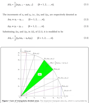
First of all, the respective triangular area is introduced. Letf(x, y) = 0 be a piecewise smooth curve of equation on thexy-plane, expressed in terms of the Cartesian coordi-nates (x, y)Î ℝ2. Assume there are two fixed points ofA(xA, yA) and B(xB, yB). Sup-pose there is a sequence of points {Pk(xk, yk) |k= 0, 1, 2, . . . ,n} onf(x, y) = 0, where the initial and the terminal points are respectively P0(x0,y0) =A(xA,yA) andPn(xn, yn) =B(xB,yB). The respective triangular area ΔSk(k= 1, 2, . . . ,n), which is surrounded by three vertices ofO(0, 0),Pk-1(xk-1,yk-1) andPk(xk, yk), is introduced as in Figure 1 by
Sk=
1
2(xkyk−1−ykxk−1) (k= 1, 2,. . .,n). (2:1)
The increments ofxkandyk, i.e.,Δxkand Δyk, are respectively denoted as
xk≡xk−xk−1 (k= 1, 2,. . .,n), (2:2)
yk≡yk−yk−1 (k= 1, 2,. . .,n). (2:3)
Substituting ΔxkandΔykinΔSkof (2.1), it is modified to be
Sk=
1
2(ykxk−xkyk) (k= 1, 2,. . .,n). (2:4)
Figure 1Sum of triangularly divided areas. The respective triangular areaΔSk, which is surrounded by
three vertices ofO(0, 0),Pk-1(xk-1,yk-1) andPk(xk, yk), is introduced as Sk=
1
2 xkyk−1−ykxk−1
Next, we introduce triangular sum Sn (n= 1, 2, 3, . . .) as a sum of ntriangular areasΔSk, i.e.,
Sn= n
k=1
Sk. (2:5)
Substituting (2.4) in (2.5), it is modified to be
Sn=
1 2
n
k=1
(ykxk−xkyk). (2:6)
Furthermore, the sum of triangular areas is modified to be the sum of a triangular area and double sums as follows. Using the notations of Δxkin (2.2) andΔykin (2.3), xkand ykare respectively expressed as
xk=x0+
k
j=1
xj (k= 1, 2,. . .,n), (2:7)
yk=y0+
k
j=1
yj (k= 1, 2,. . .,n). (2:8)
Substituting (2.7) and (2.8) in (2.6), it is finally modified to be
Sn=
1 2
n
k=1
k
j=1
xkyj−ykxj
+ 1
2(xByA−yBxA). (2:9)
The cases ofn= 1, 2, 3 andn®∞of
1 2
n
k=1
k
j=1
xkyj−ykxj
(2:10)
in (2.9) are shown in the following. Let the coordinates of pointQbe (xn, y0). 1. In the case ofn= 1, i.e., for two points ofP0(x0,y0) andP1(x1,y1) = Pn(xn, yn), it holds
1 2
1
k=1
k
j=1
xkyj−ykxj
= 0. (2:11)
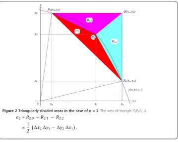
2. In the case of n= 2, i.e., for three points of P0(x0,y0),P1(x1, y1) andP2(x2,y2) =Pn (xn, yn), as shown in Figure 2, the area ofP0P1P2is
1 2
2
k=1
k
j=1
xkyj−ykxj
= 1
2(x2y1−y2x1). (2:12)
IntroducingR2.0as the area of triangleP0QPn, we obtain
R2.0=
1
2(x2−x0)(y0−y2)
=−1
2(x1+x2)(y1+y2).
IntroducingR2.1as the area of triangleP0P1Q, we obtain
R2.1=
1
2(x2−x0)(y0−y1)
=−1
2(x1+x2)y1.
(2:14)
IntroducingR2.2as the area of triangleP1P2Q, we obtain
R2.2=
1
2(x2−x1)(y0−y2)
=−1
2x2(y1+y2).
(2:15)
We introduces2as the area of triangleP0P1P2as
σ2=R2.0−R2.1−R2.2. (2:16)
Substituting (2.13), (2.14) and (2.15) in (2.16), it is modified to be
σ2=
1
2(x2y1−y2x1). (2:17)
We thus see the coincidence of (2.12) and (2.17).
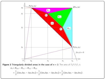
3. In the case of n= 3, i.e., for four points ofP0(x0,y0),P1(x1,y1),P2(x2,y2) and P3 (x3,y3) =Pn(xn, yn), as shown in Figure 3, the area ofP0P1P2P3 is
1 2
3
k=1 k
j=1
xkyj−ykxj=1
2(x2y1−y2x1) + 1
2(x3y1−y3x1) + 1
2(x3y2−y3x2). (2:18)
Figure 2Triangularly divided areas in the case ofn= 2. The area of triangleP0P1P2is σ2=R2.0 −R2.1 − R2.2
=1
2 x2y1−y2x1
IntroducingR3.0as the area of triangleP0QPn, we obtain
R3.0=
1
2(x3−x0)(y0−y3)
=−1
2(x1+x2+x3)(y1+y2+y3).
(2:19)
IntroducingR3.1as the area of triangleP0P1Q, we obtain
R3.1=
1
2(x3−x0)(y0−y1)
=−1
2(x1+x2+x3)y1.
(2:20)
IntroducingR3.2as the area of triangleP1P2Q, we obtain
R3.2= (x3−x1)(y0−y2)−
1
2(x3−x1)(y0−y1)− 1
2(x2−x1)(y1−y2)− 1
2(x3−x2)(y0−y2) =−1
2x2y1− 1
2x2y2− 1 2x3y2.
(2:21)
IntroducingR3.3as the area of triangleP2P3Q, we obtain
R3.3 =
1
2(x3−x2)(y0−y3)
=−1
2x3(y1+y2+y3).
(2:22)
We introduces3as the area ofP0P1P2P3as
σ3=R3.0−R3.1−R3.2−R3.3. (2:23)
Figure 3Triangularly divided areas in the case ofn= 3. The area ofP0P1P2P3is
σ3=R3.0−R3.1−R3.2−R3.3
=1
2 x2y1−y2x1
+1
2 x3y1−y3x1
+1
2 x3y2−y3x2
Substituting (2.19), (2.20), (2.21) and (2.22) in (2.23), it is modified to be
σ3= 1
2(x2y1−y2x1) + 1
2(x3y1−y3x1) + 1
2(x3y2−y3x2). (2:24)
We thus see the coincidence of (2.18) and (2.24).
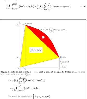
4. In the case of n®∞, i.e., for a segment of AB and a piecewise smooth curve of equation f(x, y) = 0, as shown in Figure 4, the areassurrounded by the segment and the curve is
σ = 1 2nlim→∞
n
k=1
k
j=1
xkyj−ykxj
. (2:25)
Definition 1. (Definition of a triangular integral) The triangular double integral of 1
2
[A,B]
f(x,y)≤0(dx dy−dy dx) is defined in the case of a piecewise smooth curve of
equa-tion f(x, y) = 0 by the formula,
1 2
[A,B]
f(x,y)≤0
(dx dy−dy dx) = 1 2nlim→∞
n
k=1
k
j=1
xkyj−ykxj
, (2:26)
Figure 4Single limit at infinityn®∞of double sums of triangularly divided areas. The area surrounded byf(x, y) = 0 andAB is
σ = 1 2nlim→∞
n
k=1
k
j=1
xkyj−ykxj
= 1 2
[A,B]
f(x,y)≤0
(dx dy−dy dx).
The area of the triangleOABis1
2 xByA − yBxA
wheredx’anddy’respectively correspond to increments ofΔxjandΔyj, whiledxand dy respectively correspond to those ofΔxkandΔyk.
SupposeSis the limit ofSnat infinityn®∞, i.e.,
S= lim
n→∞Sn. (2:27)
Theorem 1.The area S of OAB surrounded by OA, OB and the graph of a piecewise smooth curve of equation f (x, y) = 0is expressed as
S=1 2
[A,B]
f(x,y)≤0
(dx dy−dy dx) +1
2(xByA−yBxA), (2:28)
where O(0,0), A(xA,yA),B(xB,yB),f(xA, yA) = 0and f(xB,yB) = 0. Proof. Asn® ∞in (2.9), we obtain Sas
S= 1 2nlim→∞
n
k=1
k
j=1
xkyj−ykxj
+1
2(xByA−yBxA) (2:29)
as shown in Figure 4. Q.E.D.
Remark. The antisymmetric double integral here introduced demands only single
limit of double sums of triangularly divided areas.
2.2 Two kinds of solutions of an example of a parabola
An example that the integrand is constant is shown in Example 1. An example that the integrand is not constant is shown in Section 4.2. Two kinds of solutions of the pro-blem of a parabola are shown in the following. The first and the second solutions are respectively given by the arithmetic and the geometric sequences.
Example1. An area surrounded by a parabola of
y=−x2+ 9 (2:30)
and a segment of AB, whereA(xA,yA) = (1,8) andB(xB,yB) = (2,5). 1. Integration by the arithmetic sequence (The first kind of solution) The arithmetic sequencesxjandxkare respectively
xj= 1 +
j
n (j= 0, 1, 2, ...,k), (2:31)
xk= 1 +
k
n (k= 0, 1, 2, ...,n). (2:32)
Using (2.2), the increments of the arithmetic sequences xj andxk, i.e.,Δx =Δxj =
Δxk, are
x= 1
n. (2:33)
Substituting (2.30) in (2.3), the increments of the arithmetic sequencesyjandyk, i.e.,
yj=−
2 n−
2j−1
n2 (j= 0, 1, 2,. . .,k), (2:34)
yk=−
2 n−
2k−1
n2 (k= 0, 1, 2,. . .,n). (2:35)
Thus, the antisymmetric double increment of the arithmetic sequence (2.31) and (2.32) is
1
2(xkyj−ykxj) = k−j
n3 (j= 1, 2,. . .,k), (k= 1, 2,. . .,n). (2:36)
The double dependent sums of (2.36) forj= 1,2, . . . ,kand k= 1,2,. . . ,nis
1 2
n
k=1
k
j=1
xkyj−ykxj
= 1
n3
n
k=1
k
j=1
(k−j)
= 1 6
1− 1
n2
.
(2:37)
Asn®∞in (2.37), we obtain
1 2nlim→∞
n
k=1
k
j=1
xkyj−ykxj
= 1
6nlim→∞
1− 1
n2
= 1 6.
(2:38)
2. Integration by the geometric sequence (The second kind of solution) The geometric sequencesxjandxkare respectively
xj= 2 j
n (j= 0, 1, 2,. . .,k), (2:39)
xk= 2 k
n (k= 0, 1, 2,. . .,n). (2:40)
The increments of the geometric sequences xj, xk, yjand yk, i.e.,Δxj, Δxk, Δyjand
Δyk, are respectively
xj= 2 j
n(1−2−
1
n) (j= 0, 1, 2,. . .,k), (2:41)
yj= 2
2j n
2−2n −1
(j= 0, 1, 2,. . .,k), (2:42)
xk= 2 k
n(1−2−1n) (k= 0, 1, 2,. . .,n), (2:43)
yk= 2
2k n(2−
2
n −1) (k= 0, 1, 2,. . .,n). (2:44)
1
2 xkyj−ykxj
=1 2
1−2−1n 2−2n−1 2nk22nj−22nk2nj
(j= 1, 2,. . .,k), (k= 1, 2,. . .,n). (2:45)
The double dependent sums of (2.45) forj= 1,2, . . . ,kand k= 1, 2, . . . ,nis
1 2
n
k=1
k
j=1
xkyj−ykxj
=1 2
n
k=1
k
j=1
1−2−1n 2−2n−1 2kn22nj−22nk2nj
. (2:46)
Asn®∞in (2.46), we obtain
1 2n→∞lim
n
k=1
k
j=1
xkyj−ykxj
=1 2n→∞lim
n
k=1
k
j=1
1−2−1n 2−2n−1 2kn2
2j n −22nk2
j n
=1 6.
(2:47)
3 The combination lemma and the transformation lemma
The combination lemma is shown in Section 3.1 and the transformation lemma is shown in Section 3.2.
Lety =f(x) be a differentiable function on the xy-plane. Assume there are two fixed points ofA= (xA, yA) andB= (xB,yB) on y=f(x), whereyA=f(xA) andyB=f(xB). An ordinary integral is denoted in accordance with the notation of double integral denoted in Definition 1. New notation for an ordinary integral of y=f(x) inxÎ[xA,xB] is
[A,B]
y=f(x) y dx≡
xB
xA
f(x)dx. (3:1)
3.1 The combination lemma on the 2D plane
The combination lemma shows that the sum of an integral alongx-axis and that along y-axis between [A, B] is equal to the subtraction of two rectangles,xByBand xAyA.
Lemma 1. (The combination lemma) Assume y=f(x)is a differentiable function on the xy-plane, and x=f-1(y)is also a differentiable one, where f-1is the inverse function of f. Between A(xA,yA) = (x0, y0)and B(xB,yB) = (xn, yn),it holds
[A,B]
y=f(x) y dx+
[A,B]
x=f−1(y)
x dy=xByB−xAyA, (3:2)
where yA=f(xA)and yB=f(xB).
We name (3.2) as thecombination lemma.
Proof. It is divided into the following cases.
1. For a monotonically increasing function y=f(x) inxÎ [xA,xB] orx=f-1(y) inyÎ [yA,yB], it is indicated that the first term of the left-hand side of (3.2) is an integral of y =f(x) alongx-axis i.e.,
[A,B]
y=f(x)
y dx= lim
n→∞ n
k=1
ykxk (3:3)
[A,B]
x=f−1(y)
x dy= lim
n→∞ n
k=1
xkyk (3:4)
as shown in Figure 5.
2. For a monotonically decreasing functiony = f(x) in xÎ[xA,xB] orx = f-1(y) inyÎ [yB,yA], it holds
[B,A]
x=f−1(y)
x dy−xA yA−yB
= [A,B]
y=f(x)
y dx−yB(xB−xA) (3:5)
as shown in Figure 6. We thus obtain (3.2). Q.E.D.
3.2 The transformation lemma on the 2D plane
The transformation lemma transforms an integrand to the second integral variable. It transforms a single integral to an antisymmetric double integral of which integrand is constant.
Proposition 1.(Integral along x-axis) For a piecewise smooth curve of equation f(x, y) = 0, it holds
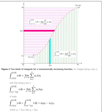
Figure 5Two kinds of integrals for a monotonically increasing function. An integral alongx-axis is
[A,B]
y=f(x)
y dx= lim
n→∞ n
k=1 ykxk
and that alongy-axis is
[A,B]
x=f−1(y)
x dy= lim
n→∞ n
k=1 xkyk.
It holds
[A,B]
y=f(x) y dx+
[A,B]
x=f−1(y)
x dy=xByB−xAyA,
[A,B]
f(x,y)=0 y dx=
[A,B]
f(x,y)≤0
dx dy+xByA−xAyA. (3:6)
Proof. Substituting (2.8) into (3.3), it is modified to be [A,B]
f(x,y)=0
y dx= lim
n→∞ n
k=1
k
j=1
yjxk+yA(xB−xA). (3:7)
Q.E.D.
Proposition 2.(Integral along y-axis) For a piecewise smooth curve of equation f(x, y) = 0,it holds
[B,A]
f(x,y)=0
x dy=−
[A,B]
f(x,y)≤0
dy dx+xAyA−xAyB. (3:8)
Proof. Substituting (2.7) into (3.4), it is modified to be [B,A]
f(x,y)=0
x dy=− lim
n→∞ n
k=1
k
j=1
xjyk+xA yA−yB
. (3:9)
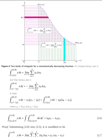
Figure 6Two kinds of integrals for a monotonically decreasing function. An integral alongx-axis is
[A,B]
y=f(x)
y dx= lim
n→∞ n
k=1 ykxk
and that alongy-axis is
[B,A]
x=f−1(y)
x dy=− lim
n→∞ n
k=1 xkyk.
It holds
[B,A]
x=f−1(y)
x dy−xA(yA−yB) = [A,B]
y=f(x)
y dx−yB(xB−xA),
Q.E.D.
Lemma 2.(The transformation lemma) For a piecewise smooth curve of equation f(x, y) = 0,it holds
[A,B]
f(x,y)=0
y dx= 1 2
[A,B]
f(x,y)≤0
dx dy−dy dx+1
2(xB−xA) yA+yB
. (3:10)
Proof. (Combining integral along x-axis with that alongy-one) Combining (3.6) with (3.8), we obtain
[A,B]
f(x,y)=0 y dx +
[B,A]
f(x,y)=0 x dy =
[A,B]
f(x,y)≤0
dx dy − dy dx + xByA − xAyB.(3:11)
Substituting (3.2) into (3.11), we obtain the lemma. Q.E.D.
4 The curl theorem of a triangular integral on the 2D plane
The curl theorem of the conventional rectangular integral (1.3) is modified to be that of a new kind of triangular integral (4.6) in Section 4.1 and its example is shown in Section 4.2.
4.1 Proof of the curl theorem on the 2D plane
We present two lemmata in the following before the proof of Theorem 2.
Lemma 3.Let X=X(x, y)be a partially differentiable function with respect to x and y. It holds
[A,B]
f(x,y)=0
X dx=1 2
[A,B]
f(x,y)≤0
∂ X
∂ydx dy
−∂X
∂ydy dx
+1
2 [A,B]
f(x,y)≤0
∂ X
∂x −
∂X
∂x
dx dx
+1
2(xB−xA)(XA+XB)
(4:1)
for a piecewise smooth curve of equation f(x, y) = 0between A(xA, yA)and B(xB,yB), where XA=X(xA,yB)and XB=X(xB, yB).
Proof. Rewriting the transformation lemma (3.10) forX =X(x, y) andf(x, y) = 0, it is expressed as
[A,B]
f(x,y)=0
X dx= 1 2
[A,B]
f(x,y)≤0
(dx dX−dX dx) +1
2(xB−xA)(XA+XB). (4:2)
Substituting two kinds of the total differentials ofX, i.e.,dX anddX’,
dX= ∂X ∂xdx+
∂X
∂ydy, (4:3)
dX= ∂X
∂xdx
+∂X
∂ydy
(4:4)
in (4.2), it is modified to be (4.1). Q.E.D.
Remark. Precise modifications in the proof of Lemma 3 are shown in Appendix 1.
[A,B]
Proof. In the similar procedure as Lemma 3, we obtain (4.5). Q.E.D.
Theorem 2.(The curl theorem of a triangular integral on the 2D plane) Let∂D be a piecewise smooth curve of equation f(x, y) = 0on the xy-plane, which is expressed in terms of the Cartesian coordinates (x, y)Î ℝ2.Let D be the region inside and on ∂D. Proof. Combining (4.1) with (4.5), we obtain
[A,B]
For an integral on a closed curve, the initial point A(xA, yA) coincides with the term-inal one B(xB,yB), i.e.,A(xA,yA) =B(xB,yB). It then holds
∂x must be rigorously distinguished as integrands. See (5.20) and
(5.19) in detail. An inequality holds for ∂X ∂x and
However, they coincide as explicit forms of derivatives. An equality holds for ∂X ∂x and ∂X
∂x in arbitrary derivative form, i.e., ∂X x,y
Corollary 1.In the case of which it holds
∂D
Xαdxα = −1
2 D
Eαβdxαdxβ, (4:11)
where indices are summed overa,b=1, 2,a sufficient condition to hold (4.11) is
−Eαβ = ∂Xα ∂xβ −
∂Xβ
∂xα (α,β = 1, 2). (4:12)
Proof. Using (4.6), (4.11) is modified to be
1 2
D
∂ Xα ∂xβ −
∂Xβ ∂xα
dxαdxβ=−1 2
D
Eαβdxαdxβ, (4:13)
where indices are summed over a, b=1, 2. A sufficient condition to hold (4.13) is (4.12). Q.E.D.
Corollary 2.In the case of (4.11), we obtain an antisymmetric property of Eabas
−Eαβ =Eβα (α,β= 1, 2). (4:14)
Proof. Interchangingaand bin (4.12), it also holds
Eβα= ∂Xα ∂xβ −
∂Xβ
∂xα (α,β= 1, 2). (4:15)
Comparing (4. 12) with (4. 15), we obtain (4. 14). Q.E.D.
4.2 An example of the curl theorem on the 2D plane
An example of Theorem 2 is shown in Example 2. The integral path of this problem is an ellipse of
x=acosθ, (4:16)
y = bsinθ. (4:17)
Definition 2. (Definition of elliptical sequence) Using (4.16) and (4.17), we may respectively introduce elliptical sequences xj, yj, xkandykas
xj=acosθj, yj=bsinθj (j= 0, 1, 2, ...,k), (4:18)
xk=acosθk, yk=bsinθk (k= 0, 1, 2, ...,n). (4:19)
The increments of xj and yj in (4.18), i.e., Δxj and Δyj, of the angular arithmetic sequenceθjare respectively
xj=a cosθj−cosθj−1
(j= 0, 1, 2, ...,k), (4:20)
yj=b sinθj−sinθj−1
(j= 0, 1, 2, ...,k). (4:21)
The increments of xk and yk in (4.19), i.e., Δxkand Δyk, of the angular arithmetic sequenceθkare respectively
yk=b(sinθk−sinθk−1) (k= 0, 1, 2, ...,n). (4:23)
Example 2. We calculate both of the line integral and the area integral in the coun-terclockwise direction. The example is the curl theorem of a triangular integral on the 2D plane in the case of X =X(x, y) = -x2y and Y= Y(x, y) = xy2, where the closed curve is an ellipse of (4.16) and (4.17).
The arithmetic sequences ofθjandθkare respectively
θj=j
1.Calculation by line integral The line integral is calculated to be
The integral in (4.27) is executed in the formula of 2π
Substituting (4.28) into (4.27), we finally obtain
2.Calculation by area integral
The area double integral in the region of x2 a2 +
Remark. It is very complicated to execute this triangular integral only by human’s brain. Computer and formula manipulation software are recommended to verify these calculations in the case ofn® ∞. This theory is also applicable for numerical calcula-tion in the case of 1 <n<∞.
5 The curl theorem of a triangular integral in the higher dimensions
The curl theorem of a triangular integral in the 3D space is derived in Section 5.1 and that in the 4D hyper-space is derived in Section 5.2.
5.1 The curl theorem in the 3D space
We extend the curl theorem of a triangular integral in the 3D space. We present three lemmata in the following before the proof of Theorem 3.
Lemma 5.Let X=X(x, y, z)be a partially differentiable function with respect to x, y and z. It holds
[A,B]
g(x,y,z)=0
X dx=1
2 [A,B]
g(x,y,z)≤0
∂X
∂ydx dy −∂X
∂ydy dx
+∂X
∂zdx dz
−∂X
∂zdz dx
+1 2
[A,B]
g(x,y,z)≤0
∂X
∂x −
∂X
∂x
dx dx+1
2(xB−xA) (XA+XB)
(5:1)
for a piecewise smooth curve of equation g(x, y, z) = 0between A(xA,yA,zA)and B(xB, yB,zB), where XA=X(xA,yA,zA)and XB=X(xB,yB,zB).
Proof. Rewriting the transformation lemma (3.10) forX=X(x, y, z) andg(x, y, z) = 0, it is expressed as
[A,B]
g(x,y,z)=0X dx=
1 2
[A,B]
g(x,y,z)≤0(dx dX−dX dx) +
1
2(xB−xA)(XA+XB). (5:2)
Substituting two kinds of the total differentials ofX, i.e.,dX anddX’,
dX= ∂X ∂xdx+
∂X ∂ydy+
∂X
∂zdz, (5:3)
dX= ∂X
∂xdx
+∂X
∂ydy
+∂X
∂zdz
(5:4)
in (5.2), it is modified to be (5.1). Q.E.D.
Lemma 6.Let Y=Y(x, y, z)be a partially differentiable function with respect to x, y and z. It holds
[A,B]
g(x,y,z)=0
Y dy= 1 2
[A,B]
g(x,y,z)≤0 ∂
Y ∂xdy dx
−∂Y
∂xdx dy
+∂Y
∂zdy dz
− ∂Y
∂zdz dy
+1 2
[A,B]
g(x,y,z)≤0 ∂
Y ∂y −
∂Y ∂y
dy dy+1
2(yB−yA)(YA+YB) (5:5)
for a piecewise smooth curve of equation g(x, y, z) = 0between A(xA,yA,zA)and B(xB, yB,zB), where YA=Y(xA,yA,zA)and YB=Y(xB,yB,zB).
Proof. In the similar procedure as Lemma 5, we obtain (5.5). Q.E.D.
[A,B]
Proof. In the similar procedure as Lemma 5, we obtain (5.6). Q.E.D.
Theorem 3.(The curl theorem of a triangular integral in the3D space) Let D be a piecewise smooth surface in the xyz-space, which is expressed in terms of the Cartesian coordinates (x, y, z)Îℝ3.Let∂D be the boundary of D. Let X1 =X = X(x, y, z), X2=Y
where indices are summed overa,b=1,2,3.
Proof. Combining (5.1) with (5.5) and (5.6), we obtain
[A,B]
5.2 The curl theorem in the 4D hyper-space
We extend the curl theorem of a triangular integral in the 4D hyper-space.
partially differentiable functions with respect to x0=t, x1 =x, x2=y and x3=z in D. It
where indices are summed overa,b=0,1,2,3. Proof. In the 4D, it holds
Using Definition 1, the first term of the right-hand side of (4.2) in the proof of Lemma 3 is expressed as
1
Xk≡X(xk,yk)−X(xk−1,yk−1)
Substituting (5.14) and (5.15) in the right-hand side of (5.13), it is modified to be
1
Each term of (5.16) is respectively expressed as
1
We thus obtain (4.1) in Lemma 3.
Appendix 2
Substituting (4.24) in (4.20) and (4.21), substituting (4.25) in (4.22) and (4.23), the respective terms of (4.30) are calculated as follows.
1. The first term of the left-hand side of (4.30) is
2. The second term of the lefthand side of (4.30) is
3. The third term of the left-hand side of (4.30) is
1
4. The fourth term of the left-hand side of (4.30) is
Acknowledgements
The author thanks to Professor Susumu Ishikawa at Fukuoka Institute of Technology for refining this theory. In the process of reviewing, the author also thanks to the referees for their instructive comments.
Competing interests
The author declares that he has no competing interests.
Received: 30 September 2011 Accepted: 2 March 2012 Published: 2 March 2012
References
1. Lebesgue, H: Intégrale, longueur, aire, Thèses présentées à la Faculté des sciences de Paris pour obtenir le grade de Docteur ès sciences mathématiques. Annali di Matematica Pura ed Applicata7(3):231–359 (1902). Bernardoni de C. Rebeschini, Milano
2. Lebesgue, H: Leçon sur L’intégration et la Recherche des Fonctions Primitives. Gauthier-Villars, Paris (1904) 3. Cartan, É: Sur l’intégration des systèmes d’équations aux différentielles totales. Annales scientifiques de 1’É.N.S..
18(3):241–311 (1901) doi:10.1186/1687-1847-2012-23
Cite this article as:Tokunaga:The curl theorem of a triangular integral.Advances in Difference Equations2012 2012:23.
Submit your manuscript to a
journal and benefi t from:
7Convenient online submission 7Rigorous peer review
7Immediate publication on acceptance 7Open access: articles freely available online 7High visibility within the fi eld
7Retaining the copyright to your article