Numerical solutions for the linear and nonlinear singular boundary value problems using Laguerre wavelets

R E V I E W

Open Access

Numerical solutions for the linear and

nonlinear singular boundary value problems

using Laguerre wavelets

Fengying Zhou and Xiaoyong Xu

*_{Correspondence: [email protected]}

School of Science, East China University of Technology, Nanchang, 330013, P.R. China

Abstract

In this paper, a collocation method based on Laguerre wavelets is proposed for the numerical solutions of linear and nonlinear singular boundary value problems. Laguerre wavelet expansions together with operational matrix of integration are used to convert the problems into systems of algebraic equations which can be efficiently solved by suitable solvers. Illustrative examples are given to demonstrate the validity and applicability of this technique, and the results have been compared with the exact solutions.

MSC: 42C40; 65D30

Keywords: Laguerre wavelets; collocation method; singular boundary value problems; operational matrix of integration

1 Introduction

Singular boundary value problems (BVPs) for ordinary differential equations occur fre-quently in the fields of engineering and science such as gas dynamics, nuclear physics, atomic structures and chemical reactions []. In most cases, we do not always find the exact solutions for the singular boundary values problems via analytical methods. In this case, it is very meaningful to give the high precision numerical solutions for this kind of problem by numerical methods.

The purpose of this paper is to develop a Laguerre wavelets collocation method as an alternative method to solve singular two-point boundary value problems of the form []

μ(x) +L xμ

_{(x) +fx,μ(x)=g(x), x∈D, ()}

subject to the following initial and boundary conditions:

Type I : μ(a) =α, μ(b) =β, ()

Type II : μ(a) =α, μ(b) =β, ()

Type III : μ(a) =α, μ(a) =β, ()

and the most general mixed boundary conditions

Type IV : aμ(a) +aμ(a) =α, bμ(b) +bμ(b) =β, ()

whereL,ai,bi,i= , ,αi,βi,i= , , ,  are known constants,Dis an open or half-open interval with endpointsaandb,f(x,μ(x)) andg(x) are continuous real valued functions onD.

Numerous research work has been invested to study the singular BVPs of the form ()-(). For more details, the reader is kindly recommended to see the survey in []. Recently, many researchers have obtained approximations for singular BVPs via various methods. For example, Kanth and Aruna applied He’s variational iteration method [], Chang em-ployed the Taylor series method [], Singh and Kumar proposed a new technique based on Green’s function [], Sahlan and Hashemizadeh used the wavelet Galerkin method [], Ar-qubet al.studied a continuous genetic algorithm [], Ebaid used the Adomian decomposi-tion method [], Gohet al.developed a quartic B-spline method [], and Nasab proposed the Chebyshev finite difference method []. Moreover, orthogonal polynomial methods have seen significant achievements in dealing with singular boundary value problems, for example, Legendre polynomials [], Chebyshev polynomials [], Bernstein polynomials [], Laguerre polynomials [], Bessel polynomials [], Hermite polynomials [], and Bernoulli polynomials []. Note that these polynomials are supported on the whole inter-val. This is obviously a defect for certain analysis work, especially problems involving local functions vanishing outside a short interval. However, one advantage of wavelet analysis is the ability to perform a local analysis. This characteristic of time-frequency localization can overcome the defect and allows us to obtain very accurate numerical solutions.

There are two different approaches for solving differential equations. One approach is based on converting differential equations into integral equations through integration, ap-proximating various signals involved in the equation by truncated orthogonal series, and using the operational matrix of integration, to eliminate the integral operations []. An-other one is based on using operational matrix of derivatives in order to reduce the prob-lem into solving a system of linear or nonlinear algebraic equations. There are some pa-pers in the literature about using the operational matrix of derivatives to solve differential equations [, , ].

The rest of this paper is organized as follows. In Section , we introduce the Laguerre wavelets and the operational matrix of integration. The error estimation of the Laguerre wavelets expansion is also given. In Section , the proposed method is used to approximate solutions of the problems. Section  gives several examples to test the proposed method. A conclusion is drawn in Section .

2 Laguerre wavelets and their properties 2.1 Wavelets and Laguerre wavelets

Wavelets constitute a family of functions constructed from dilation and translation of a single function called the mother wavelet. When the dilation parameteraand the transla-tion parameterbvary continuously, we have the following family of continuous wavelets:

ψa,b(t) =|a|–/ψ

t–b a

If we restrict the parametersaandbto discrete values asa=a–j_,b=mba–j, wherea> , b> , andj,mare positive integers, we have the following family of discrete wavelets:

ψj,m(t) =|a|j/ψ

aj_t–mb

,

which form a wavelet basis forL_{(R). In particular, whena}

=  andb= , thenψj,m(t) form an orthonormal basis.

The Laguerre waveletsψn,m(t) =ψ(k,n,m,t) have four arguments:k can assume any positive integer,n= , , , . . . , k–_{,mis the degree of Laguerre polynomials, andtis the} normalized time. They are defined on the interval [, ) as

ψn,m(t) =

k_Lm(k_{t– n+ ),} n–

k– ≤t<_kn–, , otherwise,

wherem= , , , . . . ,M–  andMis a fixed positive integer,Lm(t) are the Laguerre poly-nomials of degreemwhich are orthogonal with respect to the weight functionω(t) =e–t on the interval [,∞) and satisfy the following recursive formula:

L(t) = , L(t) =  –t, Lm+(t) =(m+  –t)Lm(t) –mLm–(t)

m+  , m= , , , . . . .

A functionμ(x)∈L_{(R) defined over [, ) may be expanded by Laguerre wavelets as}

μ(x) = ∞

n= ∞

m=

cn,mψn,m(x). ()

If the infinite series in equation () is truncated, then it can be written by

μ(x)∼= k–

n= M–

m=

cn,mψn,m(x) = CT(x),

where C and(x) are k–_{M× matrices given by}

C=c, c, · · · c,M– c, c, · · · c,M– · · · ck–_, c_k–_, · · · c_k–_,M– T

,

(x) =ψ, ψ, · · · ψ,M– ψ, ψ, · · · ψ,M– · · · ψk–_, ψ_k–_, · · · ψ_k–_,M– T

.

()

Since the truncated Laguerre wavelets series can be an approximate solution of singular BVPs, one has an error functionE(x) forμ(x) as follows:

E(x) =μ(x) – CT(x).

The following theorem gives the error estimation of the Laguerre wavelets expansion.

Theorem  Suppose thatμ(x)∈Cm_{[, ]andC}T_{(x)is the approximate solution using} Laguerre wavelets.Then the error bound would be given by

E(x) ≤ 

Proof We divide the interval [, ] into k–_{subintervalsI} By using the maximum error estimate for the polynomial onIn, we have

E(x) ≤

where we have used the well-known maximum error bound for the interpolation.

2.2 Operational matrix of integration (OMI)

In this section, we give the structure of OMI for Laguerre wavelets withk=  andM= . In this case, the six basis functions are given by

ψ,(t) = , () from  totand representing them in the matrix form, we obtain

t

Unfortunately, for generalkandM, operational matrix of integration does not have a reg-ular expression. So when dealing with the problems, we need to pre-calculate the corre-sponding operational matrix of integration P and(t) for differentkandMsuch that

t



(s)ds= P(t) +(t). ()

For example, fork=  andM= , the operational matrix of integration is given by

where A and B are × matrices given by

3 Description of the proposed method

In this section, we will use Laguerre wavelets operational matrix of integration combin-ing collocation method to solve linear or nonlinear scombin-ingular boundary value problems. Assume that

μ(x) = CT(x), ()

where C is an unknown vector which should be determined and(x) is the vector defined in (). Equation () is integrated two times with respect tox. In this way, the solutionμ(x) and its two derivatives are expressed in terms of Laguerre wavelets functions and their integrals. Consider the collocation points

xi= i– 

k_M, i= , , , . . . ,  k–_M.

The expressions ofμ(x),μ(x), andμ(x) are substituted in the given differential equa-tions and discretization is applied using the collocation points. Thus we get a system of equations with k–_Munknowns

μ(xi) + L xi

μ(xi) +fxi,μ(xi)=g(xi), i= , , , . . . , k–M. ()

Then we can obtain the unknown vector C by solving this system through the well-known Newton iterative method with the aid of Matlab. The approximate solution can easily be recovered by inserting C into the corresponding expression ofμ(x). We further explain the method with the help of specific boundary conditions. In this paper, we consider the four different types of boundary conditions ()-() and derive the expressions of μ(x),

μ(x), andμ(x), respectively. For simplicity, we takea=  andb= . Before the further description of the proposed method, we introduce the following notations first:

() := lim

Type I. Consider boundary conditions (). Assume

μ(x) = CT(x). ()

By integrating () two times with respect toxand together with relation (), we obtain

μ(x) =α+μ()x+ CT

Type II. Consider boundary conditions (). Assume

μ(x) = CT(x). ()

By integrating () two times with respect toxand by equation (), we get

μ(x) =α+ CT

Type III. Consider boundary conditions (). Assume

μ(x) = CT(x). ()

By integrating () two times with respect toxand by relation (), we obtain

μ(x) =β+ CT

Type IV. Consider boundary conditions (). Assume

By integrating () two times with respect toxand by relation (), we have

μ(x) =μ() + CTP(x) +(x), ()

μ(x) =μ() +μ()x+ CT

P(x) + P(x) +

x



(s)ds

. ()

Puttingx=  in () and () leads to

μ() =μ() + CTP() +(),

μ() =μ() –μ() – CT

P() + P() +





(s)ds

. ()

Hence equations in () turn into the following forms:

aμ() +a

μ() –μ() – CT

P() + P() +





(s)ds

=α, ()

bμ() +b

μ() –μ() – CT

P() + P() +





(s)ds

+ CTP() +()=β. ()

Observe that we considerμ() andμ() as unknown variables in equations () and (). Equations () together with () and () generate k–_{M+  equations, which can be} solved by using Newton’s iterative method.

4 Numerical examples

In order to demonstrate the efficiency and applicability of the proposed method, several linear or nonlinear singular two-point BVPs are studied. We also compare the approximate solution with the exact solution. All computations are performed by Matlab.

Example  Consider the following linear singular two-point BVP:

μ(x) +  xμ

_{(x) +} 

 –xμ(x) = cosx– xsinx+ x

 –xcosx,  <x< ,

subject to the boundary conditions

μ() = , μ() =cos.

The exact solution is given byμ(x) =x_{cosx. We solve this equation by Laguerre wavelets} collocation method withk= ,  andM= , , , , . Tables  and  show the comparison between the absolute error of exact and approximate solutions for various values ofM withk= , . As can be seen in the tables, the Laguerre wavelet solution is very close to the exact one.

Example  Consider the following nonlinear Lane-Emden equation []:

μ(x) + xμ

Table 1 Comparison of absolute errors for Example 1 (k= 2)

x Exact solution Absolute error

M = 3

Absolute error

M = 4

Absolute error

M = 5

Absolute error

M = 6

Absolute error

M = 7

0.1 0.00995004165278026 5.05015e–5 1.15174e–5 1.67248e–7 1.94092e–8 2.04877e–10 0.2 0.0392026631136497 6.99671e–5 1.49598e–5 2.08568e–7 2.37033e–8 2.44321e–10 0.3 0.0859802840213046 8.61420e–5 1.65555e–5 2.27808e–7 2.59825e–8 2.64413e–10 0.4 0.147369759040462 8.52543e–5 1.74995e–5 2.42605e–7 2.71268e–8 2.74407e–10 0.5 0.219395640472593 8.52773e–5 1.84611e–5 2.42878e–7 2.80195e–8 2.76631e–10 0.6 0.297120821367484 5.87600e–5 1.39445e–5 1.76695e–7 2.15210e–8 2.10918e–10 0.7 0.374772671769399 3.90650e–5 1.02566e–5 1.41817e–7 1.58798e–8 1.56994e–10 0.8 0.445892293982186 4.85804e–5 6.65266e–6 9.25693e–8 1.04099e–8 1.06686e–10 0.9 0.503504074299238 2.34107e–5 3.09612e–6 5.98109e–8 4.99262e–9 5.71941e–11

Table 2 Comparison of absolute errors for Example 1 (k= 3)

x Exact solution Absolute error

M = 3

Absolute error

M = 4

Absolute error

M = 5

Absolute error

M = 6

Absolute error

M = 7

0.1 0.00995004165278026 6.09766e–6 1.01327e–6 4.46956e–9 3.95315e–10 5.99699e–13 0.2 0.0392026631136497 7.11910e–6 1.19433e–6 5.22659e–9 4.73386e–10 5.69475e–13 0.3 0.0859802840213046 6.96418e–6 1.22938e–6 5.14196e–9 5.02232e–10 4.70207e–13 0.4 0.147369759040462 6.72907e–6 1.21170e–6 4.73782e–9 5.05799e–10 3.83082e–13 0.5 0.219395640472593 5.82617e–6 1.18534e–6 4.30528e–9 4.92414e–10 3.16524e–13 0.6 0.297120821367484 4.41211e–6 9.85413e–7 3.52994e–9 4.11916e–10 3.36841e–13 0.7 0.374772671769399 3.86910e–6 7.96955e–7 2.86759e–9 3.31169e–10 3.66096e–13 0.8 0.445892293982186 2.27080e–6 5.61629e–7 1.81250e–9 2.28235e–10 3.48554e–13 0.9 0.503504074299238 1.73623e–6 2.78002e–7 9.55841e–10 1.18077e–10 1.97952e–13

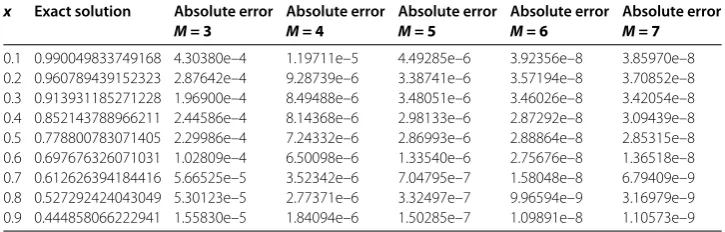
Table 3 Comparison of absolute errors for Example 2 (k= 2)

x Exact solution Absolute error

M = 3

Absolute error

M = 4

Absolute error

M = 5

Absolute error

M = 6

Absolute error

M = 7

0.1 0.990049833749168 4.30380e–4 1.19711e–5 4.49285e–6 3.92356e–8 3.85970e–8 0.2 0.960789439152323 2.87642e–4 9.28739e–6 3.38741e–6 3.57194e–8 3.70852e–8 0.3 0.913931185271228 1.96900e–4 8.49488e–6 3.48051e–6 3.46026e–8 3.42054e–8 0.4 0.852143788966211 2.44586e–4 8.14368e–6 2.98133e–6 2.87292e–8 3.09439e–8 0.5 0.778800783071405 2.29986e–4 7.24332e–6 2.86993e–6 2.88864e–8 2.85315e–8 0.6 0.697676326071031 1.02809e–4 6.50098e–6 1.33540e–6 2.75676e–8 1.36518e–8 0.7 0.612626394184416 5.66525e–5 3.52342e–6 7.04795e–7 1.58048e–8 6.79409e–9 0.8 0.527292424043049 5.30123e–5 2.77371e–6 3.32497e–7 9.96594e–9 3.16979e–9 0.9 0.444858066222941 1.55830e–5 1.84094e–6 1.50285e–7 1.09891e–8 1.10573e–9

subject to the boundary conditions

μ() = , μ() =e–.

The exact solution isμ(x) =e–x_{. We solve this equation by the proposed method with} k= ,  andM= , , , , . Tables  and  show the comparison between the absolute error of exact and approximate solutions for various values ofMwithk= , .

Example  Consider the singular initial value problem

μ(x) +  xμ

Table 4 Comparison of absolute errors for Example 2 (k= 3)

x Exact solution Absolute error

M = 3

Absolute error

M = 4

Absolute error

M = 5

Absolute error

M = 6

Absolute error

M = 7

0.1 0.990049833749168 2.08605e–4 5.07778e–7 4.15842e–7 2.78811e–9 2.71666e–9 0.2 0.960789439152323 2.21586e–4 5.87780e–7 4.10797e–7 2.80960e–9 2.51711e–9 0.3 0.913931185271228 5.48197e–5 1.20537e–6 1.38717e–7 4.74755e–9 9.86147e–10 0.4 0.852143788966211 1.92271e–5 1.45560e–6 2.03389e–8 5.53697e–9 1.07901e–10 0.5 0.778800783071405 3.85323e–5 1.36715e–6 5.24896e–8 5.19276e–9 8.98013e–11 0.6 0.697676326071031 2.41881e–5 1.19571e–6 4.21942e–8 4.19259e–9 4.05933e–11 0.7 0.612626394184416 1.59949e–5 1.01058e–6 3.36762e–8 3.38714e–9 1.56910e–11 0.8 0.527292424043049 9.22128e–6 5.95503e–7 2.06618e–8 2.03107e–9 3.88289e–11 0.9 0.444858066222941 3.14709e–6 2.04191e–7 7.61645e–9 7.32635e–10 6.69331e–11

Table 5 Comparison of absolute errors for Example 3 (k= 2)

x Exact solution Absolute error

M = 3

Absolute error

M = 4

Absolute error

M = 5

Absolute error

M = 6

Absolute error

M = 7

0.1 0.995037190209989 4.77401e–5 2.80938e–6 1.19035e–6 2.35692e–8 2.20068e–8 0.2 0.98058067569092 3.48537e–5 2.03669e–6 4.07247e–7 2.33623e–9 1.54801e–8 0.3 0.957826285221151 2.38207e–5 1.20579e–6 3.72277e–7 7.17380e–9 1.02347e–8 0.4 0.928476690885259 5.21145e–6 8.77799e–7 1.37710e–7 3.12745e–9 5.36581e–9 0.5 0.894427190999916 7.76968e–6 5.82907e–7 2.11945e–7 3.50210e–8 6.35488e–9 0.6 0.857492925712544 1.12585e–4 9.24255e–6 4.09098e–6 3.15261e–7 7.61925e–8 0.7 0.81923192051904 2.06616e–4 1.61932e–5 7.30904e–6 6.05365e–7 1.41539e–7 0.8 0.78086880944303 2.73469e–4 2.16091e–5 9.89317e–6 8.27822e–7 1.92037e–7 0.9 0.743294146247166 3.30810e–4 2.58050e–5 1.17167e–5 9.91475e–7 2.29895e–7

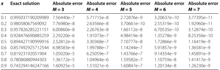
Table 6 Comparison of absolute errors for Example 3 (k= 3)

x Exact solution Absolute error

M = 3

Absolute error

M = 4

Absolute error

M = 5

Absolute error

M = 6

Absolute error

M = 7

0.1 0.995037190209989 7.56440e–7 5.71715e–8 2.72876e–9 3.20637e–10 3.77395e–11 0.2 0.98058067569092 7.76980e–8 2.63566e–8 3.70661e–10 2.55319e–10 1.92960e–11 0.3 0.957826285221151 6.00860e–8 2.26763e–8 1.66112e–8 6.70535e–10 3.12874e–10 0.4 0.928476690885259 2.29220e–6 1.91073e–7 4.98419e–8 1.35278e–9 8.25356e–10 0.5 0.894427190999916 2.52812e–6 3.30368e–7 7.10777e–8 1.72866e–9 1.16419e–9 0.6 0.857492925712544 6.98583e–6 1.99788e–7 1.14244e–7 5.91857e–9 1.36581e–9 0.7 0.81923192051904 1.05020e–5 6.25059e–7 1.43766e–7 9.14354e–9 1.45891e–9 0.8 0.78086880944303 1.36172e–5 1.04964e–6 1.59582e–7 1.10759e–8 1.41417e–9 0.9 0.743294146247166 1.60925e–5 1.51021e–6 1.60847e–7 1.20134e–8 1.26230e–9

subject to the boundary conditions

μ() = , μ() = .

The exact solution isμ(x) =√

+x. We solve this equation by the proposed method with k= ,  andM= , , , , . Tables  and  show the comparison between the absolute error of exact and approximate solutions for various values ofMwithk= , .

Example  Consider the following nonlinear Lane-Emden equation []:

μ(x) + xμ

Table 7 Comparison of absolute errors for Example 4 (k= 2)

x Exact solution Absolute error

M = 3

Absolute error

M = 4

Absolute error

M = 5

Absolute error

M = 6

Absolute error

M = 7

0.1 –0.0199006617063362 7.12293e–5 4.60723e–6 1.03881e–6 1.97866e–9 9.02739e–9 0.2 –0.0784414263065627 1.66987e–6 6.19572e–7 6.99131e–7 1.51682e–8 1.68836e–9 0.3 –0.172355392482105 1.21751e–4 1.76275e–6 3.42269e–7 2.01945e–8 6.31737e–9 0.4 –0.296840010236547 2.74878e–5 1.49126e–6 1.06726e–6 5.07048e–9 9.34269e–9 0.5 –0.44628710262842 1.06032e–5 2.81301e–6 4.23783e–8 4.20504e–8 1.76553e–10 0.6 –0.614969399495921 2.72115e–4 1.79133e–5 8.97718e–6 5.75857e–7 1.78242e–7 0.7 –0.797552239914736 4.58685e–4 2.48304e–5 1.45806e–5 9.99011e–7 2.95038e–7 0.8 –0.989392483672214 5.79446e–4 2.95584e–5 1.83900e–5 1.27201e–6 3.69959e–7 0.9 –1.18665369055547 6.57413e–4 3.25099e–5 2.04445e–5 1.43231e–6 4.14540e–7

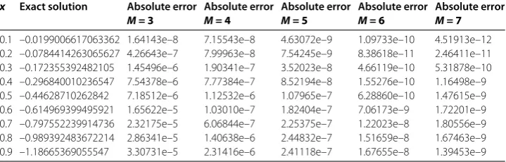
Table 8 Comparison of absolute errors for Example 4 (k= 3)

x Exact solution Absolute error

M = 3

Absolute error

M = 4

Absolute error

M = 5

Absolute error

M = 6

Absolute error

M = 7

0.1 –0.0199006617063362 1.64143e–8 7.15543e–8 4.63072e–9 1.09733e–10 4.51913e–12 0.2 –0.0784414263065627 4.26643e–7 7.99963e–8 7.54245e–9 8.38618e–11 2.46411e–11 0.3 –0.172355392482105 1.45496e–6 1.90341e–7 3.52023e–8 4.66119e–10 5.31878e–10 0.4 –0.296840010236547 7.54378e–6 7.77384e–7 8.52194e–8 1.55276e–10 1.16498e–9 0.5 –0.44628710262842 7.18512e–6 1.12532e–6 1.07965e–7 6.28860e–10 1.47615e–9 0.6 –0.614969399495921 1.65622e–5 1.03010e–7 1.82404e–7 7.06173e–9 1.72201e–9 0.7 –0.797552239914736 2.32175e–5 6.06844e–7 2.25375e–7 1.22023e–8 1.80556e–9 0.8 –0.989392483672214 2.86341e–5 1.40638e–6 2.44832e–7 1.51659e–8 1.67463e–9 0.9 –1.18665369055547 3.30731e–5 2.31416e–6 2.41118e–7 1.67655e–8 1.39453e–9

subject to the boundary conditions

μ() = , μ() = .

The exact solution isμ(x) = –ln( +x). We solve this equation by the proposed method withk= ,  andM= , , , , . Tables  and  show the comparison between the absolute error of exact and approximate solutions for various values ofMwithk= , .

Example  Consider the following linear Lane-Emden equation:

μ(x) +  xμ

_{(x) +μ(x) =x}_–x_{– x+ ,  <x< ,}

subject to the boundary conditions

μ() = , μ() = .

The exact solution isμ(x) =x–x. Next, we will give the approximate solution for this equation by the proposed method withk=  andM= . In this case, we have a linear system of six equations. By solving this system, we obtain

c,= –., c,= .,

c,= –.e–,

c,= –., c,= .,

Table 9 Comparison of absolute errors for Example 5 (k= 2, 3)

x Exact solution Absolute error

k = 2,M = 3

Absolute error

k = 2,M = 4

Absolute error

k = 3,M = 3

Absolute error

k = 3,M = 4

0.1 0.009 8.96289e–10 3.92161e–10 5.95982e–12 7.96377e–12

0.2 0.032 8.72558e–10 3.32835e–10 2.50069e–11 1.72426e–11

0.3 0.063 8.44767e–10 3.09044e–10 3.99208e–11 2.53607e–11

0.4 0.096 8.01978e–10 3.03655e–10 6.62202e–11 1.77049e–11

0.5 0.125 7.15163e–10 2.80179e–10 9.72653e–11 1.43694e–11

0.6 0.144 7.48198e–10 3.93943e–12 9.33972e–11 2.52972e–11

0.7 0.147 9.12601e–10 1.80271e–10 8.55649e–11 4.49204e–11

0.8 0.128 9.68271e–10 6.99664e–11 1.43124e–10 4.37169e–11

0.9 0.081 7.16510e–10 3.93030e–11 3.19812e–10 4.91018e–11

Table 10 Comparison of absolute errors for Example 6 (k= 2)

x Exact solution Absolute error

M = 3

Absolute error

M = 4

Absolute error

M = 5

Absolute error

M = 6

Absolute error

M = 7

0.1 0.313265850498063 2.55607e–7 8.14189e–7 1.81121e–8 1.21233e–9 3.14035e–10 0.2 0.3030154228323 4.26548e–7 8.60558e–7 1.57268e–8 1.29968e–9 3.06900e–10 0.3 0.286047265304854 1.31980e–6 8.60956e–7 1.57118e–8 1.31094e–9 2.98647e–10 0.4 0.262531127456033 8.54592e–7 8.45643e–7 1.38501e–8 1.26470e–9 2.88410e–10 0.5 0.232696783873834 5.95794e–7 8.74915e–7 1.51067e–8 1.33441e–9 2.82368e–10 0.6 0.196826805692954 4.48716e–8 6.66434e–7 1.27714e–8 1.07644e–9 2.13563e–10 0.7 0.155248106682756 2.34595e–7 4.72070e–7 7.86159e–9 7.56736e–10 1.50629e–10 0.8 0.108322763444465 9.46220e–7 3.02305e–7 5.09872e–9 4.93439e–10 9.44874e–11 0.9 0.0564386024692362 4.47318e–7 1.49726e–7 1.05906e–9 2.86694e–10 4.39479e–11

So the approximate solution is given by

μ(x) =

⎧ ⎪ ⎪ ⎪ ⎨ ⎪ ⎪ ⎪ ⎩

.×–+ .x– .x – .×–_x_{, ≤x<}

,

.×–_{– .×}–_{x+ .x}_{– .x} + .×–_x_, 

≤x≤.

Obviously, the Laguerre wavelets solution is very close to the exact solution. Table  shows the comparison between the absolute error of exact and approximate solutions for various values ofMwithk= , .

Example  Consider the following nonlinear Lane-Emden equation [, , ]:

μ(x) +  xμ

_{(x) +e}μ(x)_{= ,  <x< ,}

subject to the boundary conditions

μ() = , μ() = .

The exact solution is μ(x) = ln( – √



Table 11 Comparison of absolute errors for Example 6 (k= 3)

x Exact solution Absolute error

M = 3

Absolute error

M = 4

Absolute error

M = 5

Absolute error

M = 6

Absolute error

M = 7

0.1 0.313265850498063 1.12155e–7 7.47073e–8 7.77016e–11 2.25000e–11 1.12567e–11 0.2 0.3030154228323 1.18254e–7 7.42881e–8 7.21018e–11 2.28459e–11 1.06202e–11 0.3 0.286047265304854 8.26092e–8 6.72829e–8 1.32635e–10 1.64894e–11 9.71828e–12 0.4 0.262531127456033 7.92919e–8 5.59685e–8 1.80870e–10 5.77443e–12 8.57608e–12 0.5 0.232696783873834 3.19442e–8 4.68132e–8 2.27523e–10 2.24772e–12 7.28159e–12 0.6 0.196826805692954 1.34284e–8 3.36344e–8 2.33153e–10 8.22350e–12 5.78329e–12 0.7 0.155248106682756 6.97215e–9 2.21505e–8 2.24769e–10 1.30745e–11 4.31280e–12 0.8 0.108322763444465 3.25668e–8 1.34976e–8 1.93600e–10 1.16738e–11 2.82023e–12 0.9 0.0564386024692362 8.78766e–9 6.50385e–9 8.87945e–11 5.50390e–12 1.33990e–12

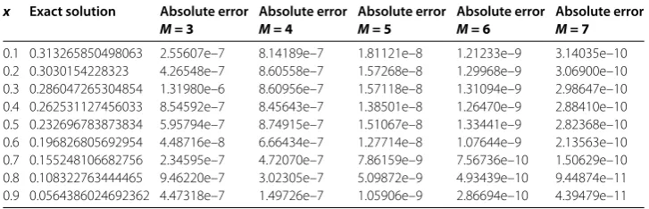
Table 12 Absolute errors for Example 6 in [16]

x Exact solution N = 10 N = 14

0.1 0.313265850498063 1.05e–7 6.69e–8 0.2 0.3030154228323 6.33e–9 7.87e–9 0.3 0.286047265304854 5.91e–8 6.92e–9 0.4 0.262531127456033 2.12e–7 2.87e–8 0.5 0.232696783873834 1.00e–8 7.40e–10 0.6 0.196826805692954 5.36e–7 6.32e–8 0.7 0.155248106682756 4.25e–8 6.95e–8 0.8 0.108322763444465 8.32e–7 3.38e–9 0.9 0.0564386024692362 4.67e–8 7.85e–8

Table 13 The numerical results of Example 7 withk= 3

x M = 3 M = 4 M = 5 M = 6 Method in [16]

withn = 14

0.1 0.829706090093794 0.82970609213969 0.829706092330806 0.829706092433877 0.82970609243390 0.2 0.833374731260013 0.833374733298822 0.833374733492775 0.833374733591078 0.83337473359110 0.3 0.839489911535405 0.839489913690883 0.8394899138631 0.83948991395376 0.83948991395381 0.4 0.848052782678684 0.848052784769831 0.848052784915137 0.848052784996097 0.84805278499617 0.5 0.85906492472985 0.859064926965802 0.859064927099445 0.85906492716925 0.85906492716933 0.6 0.872528317441265 0.872528319803658 0.872528319900291 0.87252831995828 0.87252831995828 0.7 0.888445303225948 0.888445305504435 0.888445305576983 0.888445305623171 0.88844530562329 0.8 0.906818545614923 0.906818547978651 0.906818548031817 0.906818548066776 0.90681854806690 0.9 0.927650986181403 0.927650988306455 0.927650988340659 0.927650988365551 0.92765098836568

Example  Consider the oxygen diffusion problem

μ(x) + xμ

_{(x) =} .μ(x)

μ(x) + .,  <x< ,

subject to the boundary conditions

μ() = , μ() +μ() = ,

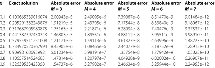
Table 14 Comparison of absolute errors for Example 8 (k= 2)

x Exact solution Absolute error

M = 3

Absolute error

M = 4

Absolute error

M = 5

Absolute error

M = 6

Absolute error

M = 7

0.1 0.100665339016074 1.99905e–4 2.28846e–5 1.72044e–6 4.80911e–7 5.02872e–8 0.2 0.205291382243876 1.91458e–4 2.34563e–5 1.63517e–6 4.79635e–7 4.89559e–8 0.3 0.317687905980875 1.67910e–4 2.28553e–5 1.57308e–6 4.65931e–7 4.71142e–8 0.4 0.441387397450343 1.61539e–4 2.17240e–5 1.47290e–6 4.39266e–7 4.45112e–8 0.5 0.579559511251008 1.51975e–4 2.13789e–5 1.36356e–6 4.18131e–7 4.14292e–8 0.6 0.734970520367994 9.83797e–5 1.29024e–5 9.77157e–7 2.95283e–7 2.86342e–8 0.7 0.909981686939921 4.84761e–5 5.13638e–6 6.43969e–7 1.71463e–7 1.62533e–8 0.8 1.10657514524663 7.88980e–6 1.98660e–6 2.77744e–7 5.15655e–8 4.25484e–9 0.9 1.32639533423358 3.47573e–5 7.91713e–6 5.42440e–8 5.87647e–8 6.74598e–9

Table 15 Comparison of absolute errors for Example 8 (k= 3)

x Exact solution Absolute error

M = 3

Absolute error

M = 4

Absolute error

M = 5

Absolute error

M = 6

Absolute error

M = 7

0.1 0.100665339016074 2.00943e–5 2.49095e–6 7.39087e–8 8.51470e–9 9.01484e–12 0.2 0.205291382243876 1.91219e–5 2.43795e–6 7.17544e–8 8.33840e–9 3.18067e–12 0.3 0.317687905980875 1.75163e–5 2.21871e–6 6.28094e–8 7.40476e–9 3.37537e–11 0.4 0.441387397450343 1.46803e–5 1.89551e–6 4.88112e–8 5.95511e–9 9.98910e–11 0.5 0.579559511251008 1.21171e–5 1.59113e–6 3.61323e–8 4.63996e–9 1.48223e–10 0.6 0.734970520367994 8.42905e–6 1.08465e–6 2.44077e–8 3.18752e–9 1.28915e–10 0.7 0.909981686939921 5.01234e–6 5.98191e–7 1.33754e–8 1.77942e–9 1.03023e–10 0.8 1.10657514524663 1.47814e–6 1.20797e–7 4.04928e–9 6.02002e–10 6.26907e–11 0.9 1.32639533423358 1.54737e–6 3.27982e–7 2.46634e–9 3.25944e–10 2.24953e–12

Example  Consider the following nonlinear singular two-point BVP:

μ(x) +  xμ

_{(x) +} μ(x)

x( –x)= arctanx+

 + x x( +x₎+

( +x₎_arctan_x

x( –x) ,  <x< ,

subject to the boundary conditions

μ() +μ() = , μ() +μ() = ..

The exact solution is μ(x) = ( +x_{)arctanx. We solve this equation by the proposed} method withk= ,  andM= , , , , . Tables  and  show the comparison between the absolute error of exact and approximate solutions for various values ofMwithk= , .

5 Conclusion

The main goal of this paper is to develop an efficient and accurate method to solve linear or nonlinear singular boundary value problems with four different types’ initial boundary conditions and mixed boundary conditions. The Laguerre wavelets operational matrix of integration together with the collocation method is utilized to reduce the problem to the solution of linear or nonlinear algebraic equations. One of the main advantages of the developed algorithm is that it does not require any modification while switching from the linear case to the nonlinear case. Another one is that high accuracy approximate solutions are achieved using very small values of k andM. Illustrative examples are included to demonstrate the validity and applicability of the proposed method.

Competing interests

Authors’ contributions

FZ and XX came up with the idea of this paper. FZ completed the proofs of the results, and XX designed a MATLAB program to simulate the results of examples. FZ and XX wrote the manuscript. All authors read and approved the final manuscript.

Acknowledgements

This work is supported by the Education Department Youth Science Foundation of Jiangxi Province (Grant No. GJJ14492), the Youth Science Foundation of Jiangxi Province (Grant No. 20151BAB211004), and the Ph.D. Research Startup Foundation of East China University of Technology (Grant No. DHBK2012205).

Received: 16 August 2015 Accepted: 11 January 2016

References

1. Kumar, M, Singh, N: A collection of computational techniques for solving singular boundary-value problems. Adv. Eng. Softw.40, 288-297 (2009)

2. Doha, EH, Abd-Elhameed, WM, Youssri, YH: Second kind Chebyshev operational matrix algorithm for solving differential equations of Lane-Emden type. New Astron.23/24, 113-117 (2013)

3. Kanth, ASVR, Aruna, K: He’s variational iteration method for treating nonlinear singular boundary value problems. Comput. Math. Appl.60, 821-829 (2010)

4. Chang, SH: Taylor series method for solving a class of nonlinear singular boundary value problems arising in applied science. Appl. Math. Comput.235, 110-117 (2014)

5. Singh, R, Kumar, J: An efficient numerical technique for the solution of nonlinear singular boundary value problems. Comput. Phys. Commun.185, 1282-1289 (2014)

6. Sahlan, MN, Hashemizadeh, E: Wavelet Galerkin method for solving nonlinear singular boundary value problems arising in physiology. Appl. Math. Comput.250, 260-269 (2015)

7. Arqub, OA, Abo-Hammour, Z, Momani, S, Shawagfeh, N: Solving singular two-point boundary value problems using continuous genetic algorithm. Abstr. Appl. Anal.2012, Article ID 205391 (2012)

8. Ebaid, A: A new analytical and numerical treatment for singular two-point boundary value problems via the Adomian decomposition method. J. Comput. Appl. Math.235, 1914-1924 (2011)

9. Goh, J, Majid, AA, Ismail, AIM: A quartic B-spline for second-order singular boundary value problems. Comput. Math. Appl.64, 115-120 (2012)

10. Nasab, AK, Kılıçman, A, Atabakan, ZP, Leong, WJ: A numerical approach for solving nonlinear Lane-Emden type equations arising in astrophysics. New Astron.34, 178-186 (2015)

11. Pandey, RK, Kumar, N, Bhardwaj, A, Dutta, G: Solution of Lane-Emden type equations using Legendre operational matrix of differentiation. Appl. Math. Comput.218, 7629-7637 (2012)

12. Pandey, RK, Kumar, N: Solution of Lane-Emden type equations using Bernstein operational matrix of differentiation. New Astron.17, 303-308 (2012)

13. Gürbüz, B, Sezer, M: Laguerre polynomial approach for solving Lane-Emden type functional differential equations. Appl. Math. Comput.242, 255-264 (2014)

14. Parand, K, Nikarya, M, Rad, JA: Solving non-linear Lane-Emden type equations using Bessel orthogonal functions collocation method. Celest. Mech. Dyn. Astron.116, 97-107 (2013)

15. Öztürk, Y, Gülsu, M: An approximation algorithm for the solution of the Lane-Emden type equations arising in astrophysics and engineering using Hermite polynomials. Comput. Appl. Math.33, 131-145 (2014)

16. Mohsenyzadeh, M, Maleknejad, K, Ezzati, R: A numerical approach for the solution of a class of singular boundary value problems arising in physiology. Adv. Differ. Equ.2015, Article ID 231 (2015)

17. Yousefi, SA: Legendre wavelets method for solving differential equations of Lane-Emden type. Appl. Math. Comput.

181, 1417-1422 (2006)

18. Nasab, AK, Kılıçman, A, Babolian, E, Atabakan, ZP: Wavelet analysis method for solving linear and nonlinear singular boundary value problems. Appl. Math. Model.37, 5876-5886 (2013)

19. Kaur, H, Mittal, RC, Mishra, V: Haar wavelet approximate solutions for the generalized Lane-Emden equations arising in astrophysics. Comput. Phys. Commun.184, 2169-2177 (2013)

20. Mehrpouya, MA: An efficient pseudospectral method for numerical solution of nonlinear singular initial and boundary value problems arising in astrophysics. Math. Methods Appl. Sci. (2015). doi:10.1002/mma.3763 21. Khuri, SA, Sayfy, A: A novel approach for the solution of a class of singular boundary value problems arising in