Sink mobility aware energy efficient network integrated super heterogeneous protocol for WSNs

(1)

R E S E A R C H

Open Access

Sink mobility aware energy-efficient

network integrated super heterogeneous

protocol for WSNs

Mariam Akbar

1

, Nadeem Javaid

1*

, Muhammad Imran

2

, Naeem Amjad

1

, Majid Iqbal Khan

1

and Mohsen Guizani

3

Abstract

In this paper, we propose Balanced Energy-Efficient Network Integrated Super Heterogeneous (BEENISH), improved BEENISH (iBEENISH), Mobile BEENISH (MBEENISH), and improved Mobile BEENISH (iMBEENISH) protocols for

heterogeneous wireless sensor networks (WSNs). BEENISH considers four energy levels of nodes and selects cluster heads (CHs) on the base of residual energy levels of nodes and average energy level of the network, whereas iBEENISH dynamically varies the CHs selection probability in an efficient manner leading to increased network lifetime. We also present a mathematical sink mobility model and validate this model by implementing it in BEENISH (resulting in MBEENISH) and iBEENISH (resulting in iMBEENISH). Finally, simulation results show that BEENISH, MBEENISH, iBEENISH, and iMBEENISH protocols outperform contemporary protocols in terms of stability period, network lifetime, and throughput.

Keywords: Mobility management, Clustering, Heterogeneous, WSNs, Energy efficient, Routing, Super heterogeneous

1 Introduction

A wireless sensor network (WSN) is a collection of small sized sensors (nodes) which are deployed in the area of interest. These nodes are able to sense different param-eters and can communicate with each other as well as communicate with the sink (also called base station (BS)). These nodes operate on small batteries and have limited processing and limited wireless communication capabili-ties [1, 2]. Nodes are independent when deployed in the field because they are able to self-configure and survive. However, it is difficult to re-charge them. So, energy con-sumption of these nodes should be minimum in order to achieve an appreciable network lifetime. Routing proto-cols play a key role in achieving longer network lifetime. To achieve fault tolerance, usually, WSNs consist of hun-dreds or even thousands of sensor nodes [3–5]. WSNs are used in a variety of applications such as military surveillance, patient monitoring, environmental monitor-ing, traffic transportation, and vibration monitoring [6].

*Correspondence: [email protected]

1COMSATS Institute of Information Technology, Islamabad, Pakistan Full list of author information is available at the end of the article

Considering the reduced capabilities of nodes, commu-nication with the BS could be conceived without routing protocols. With this assumption, the flooding technique [7] becomes prominent due to its simplicity in imple-mentation. In this technique, a source node initiates a data broadcast. Consecutive retransmissions of the source data by neighboring nodes are then made to ensure data delivery at the intended destination. However, this imple-mentation simplicity brings about many drawbacks: nodes receive multiple copies of the same data, different nodes transmit copies of the same data, nodes have limited resources but these do not limit their functionalities, etc. In order to overcome these drawbacks, gossiping [8] has been introduced. Instead of transmitting data to all neigh-bors, the gossiping technique transmits data to selected neighbors. This technique avoids implosion; however, resource blindness and overlapping are still present. More importantly, these drawbacks become more prominent as the node density is increased. Due to drawbacks in exist-ing techniques, development of energy-efficient routexist-ing protocols is very much necessary now. Soon after network establishment, routing protocols take charge of construct-ing as well as maintainconstruct-ing routes between nodes and the

(2)

Akbaret al. EURASIP Journal on Wireless Communications and Networking (2016) 2016:66 Page 2 of 19

BS. The ways in which routing protocols perform route discovery and maintenance make these protocols suitable for certain applications.

WSNs are of two types: homogeneous and heteroge-neous. In the first type, all nodes when deployed in the network are initially equipped with the same energy levels. However, in the second type, nodes before the start of network operation are equipped with different energy levels. Low Energy Adaptive Clustering Hierar-chy (LEACH) [9] and Hybrid Energy-Efficient Distributed (HEED) protocols [10] are clustering routing protocols which are especially designed for homogeneous WSNs. As a consequence, these schemes do not perform well in het-erogeneous networks, since they are designed solely for homogeneous environments. On the other hand, in het-erogeneous environments, LEACH and HEED are unable to discriminate between nodes with high energy (that is, they have a longer lifetime) and nodes which posses low energy (die more quickly). On the other hand, cluster-ing protocols for heterogeneous environments are effi-ciently designed to tackle heterogeneity in the network [4, 5]. Smaragdakis et al. [11] proposed a Stable Elec-tion Protocol (SEP) for two-level heterogeneous WSNs. SEP considers two types of nodes according to their initial energies: normal and advanced. Advanced nodes are equipped with more energy than the normal ones. Distributed Energy-Efficient Clustering (DEEC) [12] and Developed DEEC (DDEEC) [13] start from two energy levels, whereas Enhanced DEEC (EDEEC) [14] starts from three energy levels. Afterwards, these three approaches will be generalize to support multi-energy levels.

In this paper, we propose BEENISH protocol, where a network has four different energy levels of nodes: nor-mal, advanced, super, and ultra-super. In this scheme, normal nodes have the less initial energy level as com-pared to ultra-super nodes that have the highest initial energy level. Following the same principle as of LEACH and DEEC, BEENISH rotates the CHs among nodes. In BEENISH, selection of CHs follow the probability that is the ratio between residual energy of each node and aver-age energy of the network. Based on the residual energy, BEENISH chooses different epochs for each of the nodes. Nodes with higher energy are more often selected as CHs as compared to the lower energy ones. In some cases, ultra-super, super, and advanced nodes are more punished than the normal ones in BEENISH. iBEENISH solves this problem by dynamically adjusting the CH selection proba-bility. Results show that BEENISH and iBEENISH achieve longer stability periods, enhanced network lifetime, and increased number of messages sent to the BS as compared to DEEC, DDEEC, and EDEEC, respectively. The sink mobility version of the proposed BEENISH and iBEEN-ISH perform better than the non-sink mobility versions in terms of the selected performance evaluation parameters.

This work is an extension of our previously published protocol BEENISH [15].

The remainder of this paper is organized as follows. Section 2 presents the related work. Section 3 presents the four-level heterogeneous WSN model. Our proposed routing schemes are described in Section 4. Section 5 contains the sink mobility model. Section 6 illustrates the simulation results. Section 7 concludes our research work.

2 Related work

In order to achieve energy efficiency at the network layer in WSNs, many routing protocols have been proposed (Table 1). These protocols decide the routing path for delivering the data to the end station [16]. Generally, rout-ing protocols can be divided into three categories: (i) flat routing protocols, (ii) cluster-based routing protocols, and (iii) location-based routing protocols. Nodes perform sim-ilar tasks, there exists no structure for routing, nodes are connected, and they forward data through connected nodes, in the first category of routing protocols. Whereas in the second category, network is divided into clusters and nodes select CH and send data through CH. As the name indicates, the third category exploits nodes’ location for routing. Among these categories, cluster-based rout-ing protocols are the most energy-efficient ones. There-fore, category number two is our focal point in this research work.

Heinzelman et al. [9] introduced a clustering algorithm for homogeneous WSNs; LEACH, which is based on probability nodes, select themselves as CHs. They divide the protocol operation into two phases: setup phase and steady state phase. In the setup phase, two tasks are performed: selection of CHs and association of cluster members with CHs. Every node generates a random num-ber (between 0 and 1) and compares this random numnum-ber with a pre-defined threshold value. If the generated ran-dom number is greater than the pre-defined threshold value and the node has not been selected as CH for the last

1

p rounds (pis the probability of CH selection), then it is

selected as the CH for the current round. The CH node(s) sends an association message to the non-CH nodes to inform them that it is the CH now. On reception, the non-CH nodes respond to the nearest CH node by send-ing a confirmation message. Soon after the setup phase, the steady state phase begins with data transmission from nodes to CHs and then from CHs to the BS. All these transmissions and receptions are performed within the allocated Time Division Multiple Access (TDMA) slots while keeping in mind that these allocations are centrally controlled by the BS.

(3)

Journal

LEACH [9] Clustering algorithm Homogeneous WSNs Transmissions and receptions within the allocated TDMA only, cluster heads are elected randomly hence optimal number and distribution of cluster heads cannot be ensured and cannot be used with large-scale WSNs

Better network lifetime, high data delivery ratio

HEED [10] Hybrid but fully distributed clustering scheme

Multi-hop WSN clustering algorithm

More CHs are generated than the expected number and this accounts for unbalanced energy consumption in the network, significant overhead in the network causes noticeable energy dissipation resulting in lower network lifetime

Uniform CH distribution across the network and load balancing; multi-hop fashion between the CHs and the BS promote more energy conservation and scalability

SEP [11] Hierarchically clustered scheme

Heterogeneous network for WSNs

Supports only static nodes, does not support more than two levels of hierarchy in terms of energy

Weighted election probability for becoming a CH, longer stability period scalable

DEEC [12] Clustering-based algorithm

Heterogeneous aware network for WSNs

Overhead and complexity of forming clusters in multiple levels implementing threshold-based functions

CH selected on the basis of probability of ratio of residual energy and average energy of the network, a node having more energy has more chances to be a CH. It prolongs the lifetime of the network

DDEEC [13] Energy-aware adaptive clustering based algorithm

As the initial energy of nodes is reduced and as time passed by, advanced nodes will have the same CH selection probability like the normal ones.

Permits to balance CH selection on the basis of residual energy, a node having more energy has more chances to be a CH. It prolongs the lifetime of the network.

EDEEC [14] Energy-aware adaptive clustering-based algorithm

3 types of nodes involved, more level of complexity involved More data packets received at base station, a node having more energy has more chances to be a CH. It prolongs the lifetime of the network and the stability period.

BEENISH [15] Multi-level energy-based scheme

4 types of nodes involved, more level of complexity involved, ultra-super, super, and advanced nodes are more punished than the normal ones

Longer stability periods, enhanced network lifetime increased number of messages sent to the BS

EDR [16] Data routing scheme Data centric routing for WSNs Limited to data centric routing, does not support cluster-based routing, improper load balancing

Ability to use in both event-driven and query-driven applications, ensuring shortest, routing path, transmitting very less number of packets, significant power savings

EACLE [17] Tree-rooted distributed clustering scheme

Transmission power controlled WSNs

Does not support outdoor wireless channel model, only a single sink for hundred of sensors deployed

Avoids packet collision, facilitates packet binding, energy-efficient

HRLS [19] Hierarchical location service based scheme

Practical distributed location serviced WSNs

More energy is consumed in the computation processes Provides sink location information in a scalable and distributed manner, each sink in HRLS distributively constructs its own hierarchy of grid rings

TTDD [23] Geographic routing-based scheme

Low power scheme WSNs for efficient data delivery

Forwarding path is not the shortest path and may lead to large latency for longer path; grid structure formation and query flooding cost large energy consumption

(4)

Akbar

et

al.

EURASIP

Journal

o

n

W

ireless

C

ommunications

and

Networking

(2016) 2016:66

Page

4

o

f

1

9

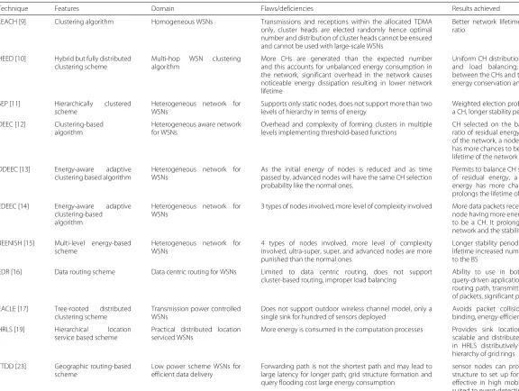
Table 1Comparison of the state-of-the-art work(Continued)

Technique Features Domain Flaws/deficiencies Results achieved

DLA [27]] Localization-based scheme

Spatially constrained WSNs More energy is consumed in the computation processes Position estimation performed by each node in an iterative manner, constraints enable nodes to update their positions on regular intervals; for reducing energy consumption, a stopping criteria for wireless transmissions has been introduced

VGDRA [28] Grid-based dynamic scheme

Dynamic route adjustment technique for WSNs

Only a few nodes are able to adjust their data routes for data delivery

(5)

power, which shortens the lifetime of the WSNs. To cope with this problem, the authors proposed a clustering-based routing protocol Power Aware Routing and Clus-tering (PARC) Scheme for WSNs which reduces these overheads.

HEED [10] is a distributed clustering algorithm which stochastically selects the CHs. This hybrid approach selects CHs on the basis of probability and minimizes the energy cost by association mechanism. This algorithm exploits the availability of multiple transmission power levels of nodes and correlates the selection probability of each node to its residual energy.

In [18], authors proposed a novel method for mobile sink operations in which the probe priority of the mobile sink is determined from data priority to increase the QoS. They use the mobile sink to reduce the routing hot spot.

In the SEP protocol proposed in [11], every protocol in which every sensor node in a heterogeneous two-level hierarchical network independently selects itself as a CH based on its initial energy.

Qing et al. [12] proposed the DEEC protocol in which the CH selection is based on the probability of the ratio of residual energy of nodes and the average energy of the network. In this algorithm, a node with a higher energy has more chances to be selected as CH.

The DDEEC, proposed in [13], selects CHs on the basis of residual energy of nodes. Thus, this process makes the advanced nodes more probable to be selected as CHs dur-ing the initial rounds as compared to the normal nodes. As the initial energy of nodes is reduced and as time passed by, advanced nodes will have the same CH selection prob-ability like the normal ones.

Saini and Sharma [14] proposed the EDEEC proto-col which extends the concept of heterogeneity to three energy levels by adding the concept of super nodes.

Authors in [19] introduced the Hierarchical Ring Loca-tion Service (HRLS) protocol, a practical distributed loca-tion service which provides sink localoca-tion informaloca-tion in a scalable and distributed manner. In contrast to existing hierarchical-based location services, each sink in HRLS distributively constructs its own hierarchy of grid rings.

In [20], authors proposed a new independent structure-based routing protocol which implements a sink mobility and provides scalability by exploiting k-level indepen-dent grid structure for data dissemination from source to destination. However, independent of the number of movement of both sinks and events, the propped protocol does not construct any additional routing structure.

Zhao et al. [21] proposed a framework to maximize the lifetime of WSNs by using a mobile sink. They formulated linear programming models for static as well as mobile sinks. Within a predefined delay tolerance level, each node does not need to send the data immediately as it becomes available. Instead, a node can store data temporarily and

transmit it when the mobile sink arrives at the most favor-able location for achieving extended network lifetime.

Authors in [22] focused on the upper bound of the total distance traveled by the mobile sink. Authors believe that the inter-transition distance between any two successive positions of a mobile sink must be restricted to avoid data loss. Also, considering the overhead on a routing tree con-struction at each sojourn location of the mobile sink, it is required that the mobile sink sojourns for at least a certain duration at each of its sojourn locations.

In [23], Luo and Hubaux jointly considered sink mobility and routing to maximize data collection during the net-work lifetime. However, authors in [21–23] do not exploit clustering, whereas we do so in order to prolong the net-work lifetime. Mobility of actors has been exploited in [24–26] to improve or recover connected coverage lost due to failure of an actor.

A distributed localization technique has been presented in [27] for WSNs. In this technique, position estimation is performed by each node in an iterative manner by solv-ing spatially constrained local programs. On the bases of range and estimated position(s), the defined constraints enable the nodes to update their positions on regular intervals. In order to reduce energy consumption of the network, a stopping criteria for wireless transmissions has been introduced.

A Virtual Grid-Based Dynamic Routes Adjustment (VGDRA) scheme is presented in [28]. It minimizes the remonstration cost of routes and maintain optimal routes near the mobile sink stop. They design set of rules for communication through which few nodes adjust their routes for data delivery. Through this strategy, they min-imize the energy consumption of remaining nodes. As a result, this scheme improves network lifetime as com-pared to the existing schemes.

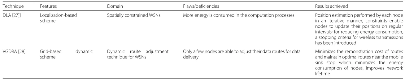
Our proposed scheme is a hybrid that utilizes the ben-efits of both clustering and sink mobility. To maximize the network efficiency, we consider a four-level hetero-geneous network, where the network field is divided into clusters. Cluster formation method and CH selection cri-teria are defined in the next sections. The CH that has minimum energy, mobile sink stops on its location and directly gathers data from nodes. In this way CH mini-mizes the energy consumption and stays alive for a longer time.

3 Four-level heterogeneous WSN model

A WSN can have nodes with different initial energies. Such kind of network is heterogeneous where initial ener-gies of nodes are different. In our proposed scheme, we consider four different energy levels of nodes. On the bases of their energy, we call them normal, advanced, super, and ultra-super. Where normal nodes’ energy isE0,

(6)

network, and their energy isa times more than that of the normal ones, i.e.,E0(1+a). Super nodes have greater

energy as compared to the advanced nodes and they are of fractionm0of normal nodes with energybtimes greater

as compared to normal nodes,E0(1+b). Similarly,

ultra-super nodes are of fraction m1 of normal nodes with u

times more energy than normal nodes,E0(1+u). Total

number of ultra-super nodes presented in the network are calculated as follows:

Total_Numultra_super=Nm1 (1)

where N is the total number of nodes in the network. Super nodes in the network are calculated as

Total_Num_super=Nm0 (2)

Advanced nodes in the network are computed by

Total_Numadvanced =Nm (3)

Whereas normal nodes are calculated as follows:

Total_Numnormal=N(1−m1−m0−m) (4)

Initial energy of the ultra-super nodes is calculated as follows:

Eultra_super=Totalultra_super×E0(1+u)=Nm1E0(1+u) (5) Initial energy of the super nodes is calculated as follows:

Esuper=Totalsuper×E0(1+b)=Nm0E0(1+b) (6) The total initial energy of all advanced nodes is computed by

Eadvanced=Totaladvanced×E0(1+a)=NmE0(1+a) (7) Initial energy of the normal nodes is calculated as follows: Enormal=Totalnormal×E0=N(1−m1−m0−m)E0 (8) Initial energy of the heterogeneous network is computed by adding the energies of normal, advanced, super, and ultra-super nodes. The total initial energy is given in Eqs. (9) and (10) as follows:

Etotal=Eultra_super+Esuper+Eadvanced+Enormal (9)

Etotal=Nm1E0(1+u)+Nm0E0(1+b)

+NmE0(1+a)+N(1−m1−m0−m)E0

(10) As compared to the homogeneous network with initial energy E0, our proposed heterogeneous WSN contains

Nm1(1+u)+Nm0(1+b)+Nm(1+a)+N(1−m1−m0−m)

times more energy. Both networks have equal number of nodes. Figure 1 presents the network model of BEENISH

When the network starts operation, nodes consume different amounts of energy for transmission depending upon the distance. Moreover, as compared to the nodes in the cluster, CH has more load of transmission, as it

receives the data from member nodes and sends it to BS. In this way, CHs consume more energy. After some time, the residual energy of nodes present in the network may vary. We conclude that after a certain time (rounds), a homogeneous system becomes heterogeneous because of difference in residual energy of nodes.

4 Proposed schemes: BEENISH and iBEENISH

This section presents the brief overview of our proposed scheme BEENISH, then we describe iBEENISH. Selec-tion criterion of CHs in BEENISH considers the residual energy of nodes and the average energy level of the net-work. Moreover, BEENISH considers a heterogeneous network with four different energy level nodes (i.e., nor-mal, advanced, super, and ultra-super).

Rotating epoch is defined withnithat represents

num-ber of rounds for a nodesiin which it can become a CH,

wherei= 1, 2, ....N. Energy consumption of CH (node) is greater than member nodes in a cluster. Ifpoptrepresents

the optimal probability for the selection of CHs in a homo-geneous network, then poptN is the number of CHs per

round are ensured on average.ni is defined asni = _p_opt1 ,

in which each nodesi atleast once becomes CH. We are

considering different energy levels among nodes, so when network operation starts, it follows LEACH criteria and epochniis kept constant for all nodes. Due to which there

is non-uniform energy distribution. Low energy node can be selected as CH and drains its energy. As a result, less energy nodes die before the nodes with greater energy. To overcome this deficiency, BEENISH rotates the epoch on the basis of nodes’ residual energy levels,Ei(r). As a result,

energy consumption is balanced because initially nodes with high energy have high residual energy and they are frequently selected as CHs as compared to normal ones. More specifically, ultra-super nodes have high frequency to become CH as compared to rest of the three levels. After that, super nodes are more frequently selected as CH as compared to the remaining two levels. Similarly, normal nodes have less frequency of becoming CH as compared to the advanced nodes. In this way, the load distribution on each node is almost uniform.

Let for epochni, pi = _n1_i defines the probability of a

node to become a CH. Our proposed scheme chooses the average probabilitypito bepoptwhich ensures that there

arepoptnumber of CHs in each round. Hence, all nodes

die at approximately the same time. If the energy levels of nodes are different, thenpi>poptfor high energy nodes.

¯

E(r)represents the average energy of the network dur-ing therthround [12]. It is calculated as follows:

¯ E(r)= 1

NEtotal

1− r R

(11)

(7)

Fig. 1Network topology of BEENISH

R= Etotal Eround

(12)

where Eround is the network’s energy consumption per

round and is calculated as

Eround=L

2NEelec+NEDA+kεmpd4toBS+Nεfsd2toCH

(13)

where the number of clusters in every round are denoted byk, CH pays cost in the form of data aggregation energy EDA, distance between CH and BS is represented bydtoBS,

whereas, distance between node in a cluster and CH is dtoCH. IfNnodes are randomly deployed in anM2region,

then

dtoCH=

M √

2πk,dtoBS=0.765 M

2 (14)

The value of kopt (that is optimal number of clusters in

the network) is given below. It is calculated by taking the derivative ofEroundwith respect tokand setting it equal

to zero.

kopt=

√ N √

2π

εfs

εmp

M

d_toBS2 (15)

The value of threshold probability is calculated in the same manner as authors did in [9, 12]. Based on this value, a nodesi decides whether to become a CH or not. The

threshold probability is given below:

T(si)=

pi

1−pi

rmod_Pi1

ifsiG

0 otherwise

(16)

whereGis the set of nodes which are eligible to be selected as CHs. SetGrepresents the nodes that do not become CH. These nodes choose a random number between 0 and 1. Then they compare chosen number to the threshold T(si), if number is less than threshold value then nodesi

becomes CH for that particular round.

(8)

with different initial energies (normal, advanced, super and ultra-super nodes). CH selection probability of nor-mal, advanced, super and ultra-super is given below:

pBEENISH_i =

The above expression shows that a node with high resid-ual energy has high probability of becoming CH. This strategy is energy efficient and distributes the load among the nodes in a balanced manner. As a result, stability period of the network increases. As it is possible that at some stages during the network lifetime three types of greater energy nodes (ultra-super, super, and advanced) have the same energy as that of normal nodes, in this case, ultra-super nodes have high frequency to be selected as CH and they are penalized more than super and advanced nodes. Similarly, in comparison to advanced nodes, super nodes are more penalized. To avoid this conventional approach for selecting CH, in the proposed scheme, prob-ability of nodes to become CH varies with the varying residual energy. Implementing the above mentioned strat-egy of frequently penalizing the nodes with higher resid-ual energies balances energy consumption resulting in smooth behavior of the proposed schemes.

In this regard, our proposed iBEENISH protocol makes some changes in the probabilities defined in the BEENISH protocol. The difference is based on the absolute resid-ual energyTabsolute, which varies the probability according

to variation in the residual energy. If ultra-super, super, and advanced nodes drain their energies and their resid-ual energy become eqresid-ual to the same energy level as that of normal nodes, then the probability of becoming a CH varies and all four kind of nodes will have the same proba-bility. The selection probabilities of nodes to become CHs in iBEENISH are given in Eq. (18):

Absolute residual energy level is denoted byTabsoluteand

its value is given in Eq. (19):

Tabsolute=zE0 (19)

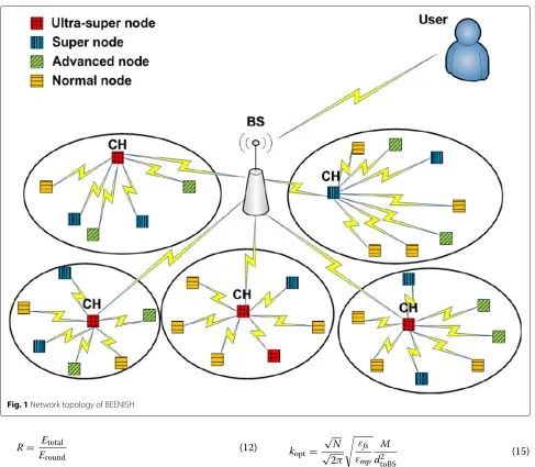
where the value of z lies in the range of [ 0, 1]. If z = 0 and Tabsolute = 0, then the scheme working behind

is BEENISH. We run the simulation many times vary-ing the value of z. The value of z = 0.71 is showing best results. The main objective is to obtain longer sta-bility period. It is observed that it is not necessary that all nodes with a higher energy level become CH. There is always an optimal number of CHs in the network. Some-times, it is also probable that normal nodes become CH. In Fig. 2, we obtain best results for first dead node using the parameters given in Table 2.

Tabsolute=0.71×E0 (20)

Through valuec, the number of CHs are optimized and it is a positive integer. For both smaller and larger values ofc, our scheme works in a “direct communication” man-ner. The reason behind this is that the majority of nodes send their data directly to the BS. In direct communica-tion, nodes send their data directly to BS. The nodes that are far from the BS consume more energy in long-distance transmissions. In order to avoid long-distance communi-cation, we find the optimum value ofcwhich provides the best results in terms of the death of the first node. For this purpose, we run simulations many times by varying value of cbetween range [0, 1] and find that atc = 0.02 net-work shows better results in terms of the death of the first node; Fig. 2 shows howcaffects the round in which the first node dies.

5 Sink mobility

The energy efficiency is the main objective in any WSN so that the network lifetime and stability period can be maximized. Nowadays, sink mobility is an effective way to maximize the network lifetime and stability period of the network. So, we introduce sink mobility in BEENISH and iBEENISH protocols and then examine their effects. We put a greater emphasis on the network stability period

(9)

Fig. 2Variation round ofcandzuntil the first node dies

because a greater stability period gives better and reliable data.

Sink mobility is divided into two classes: un-controlled and controlled mobility. In the first technique, the sink is able to move freely/randomly in the network, whereas, in the second technique, the sink can follow only pre-defined path throughout the network lifetime. Furthermore, con-trolled mobility is of two types. The first one is non-adaptive and non-flexible, which chooses fixed sojourn locations of the sink for the whole network lifetime, whereas the second technique is adaptive, robust, and flexible because it chooses sojourn locations for mobile sink in every round in order to maximize the network lifetime. We implement this adaptive technique.

When the sink is static, the probability of getting cov-erage holes in the network increases. After some time, when network is operational, the energy of few nodes in

Table 2Simulation parameters

Parameter Value

Network field 100 m×100 m

Number of nodes 100

E0 0.5 J

Message size 4000 bits

Eelec 50 nJ/bit

Efs 10 nJ/bit/m2

Eamp 0.0013 pJ/bit/m4

EDA 5 nJ/bit/signal

d0(threshold distance) 70 m

popt 0.1

the network possibly becomes low which can lead toward a coverage hole problem. Coverage holes are avoided in WSN because those regions where nodes die are left unat-tended and then it becomes difficult to monitor. Sink mobility effectively minimizes the generation of cover-age holes and balances the energy consumption among the sensors. This is why we implement sink mobility in BEENISH and iBEENISH and improve the stability period of both of them. Sink mobility versions of BEENISH and iBEENISH are MBEENISH and iMBEENISH, respectively.

5.1 System model

In our system model, the network follows the following assumptions:

1. The considered WSN is proactive. All nodes in the network generate equal amount of data per unit time. 2. Each data unit is of the same length.

3. All nodes have the same transmission range. 4. Each node has a unique pre-defined ID.

5. Protocol operation has rounds that are equal time slots.

6. At the beginning of each round, new sink locations are computed which remain fixed during that round. 7. Sinks have no energy constraint and able to move

from one sink location to another.

8. Sink moves to a location outside the network for recharging fuel or electricity.

5.2 Issues to be tackled in sink mobility

(10)

When a mobile sink moves from one sink location to another, the probability of data loss is high; so, the distance between two sink locations should be at minimum. Adap-tive sink mobility requires that the sink must re-construct the routing table or routing tree at each new location, which takes a specific time. So, a mobile sink should reside for a minimum amount of time at each sink location. The transmission of data from nodes/CHs to a sink only occurs when the sink is not moving, i.e., sink is located at any sink location. Therefore, the sum of stop times in a mobile sink tour should be maximized. There should be a max-imum number of stop locations for a mobile sink so that the throughput is maximized.

Another important issue that we elaborate on here is the use of sink mobility in a clustered environment. Most of the recent research works implement sink mobil-ity in cluster-less topologies. The reason behind this is non-compatibility between clustering and sink mobility. If we apply the same sink mobility in a clustered envi-ronment and a cluster-less envienvi-ronment taking all other parameters constant, the comparison shows that the net-work lifetime and stability period of a cluster-less protocol is much better than the clustered protocol. We tackle this issue efficiently and implement the sink mobility in our clustered heterogeneous protocol MBEENISH and iMBEENISH that results in prolonged network lifetime and extended stability period [29].

5.3 Mobile sink model

In this subsection, we propose a mathematical model of sink mobilitymobile sink model(MSM) in which we take a single sink that can move to certain sink locations in every round. Sink locations are determined at the start of every round in our proposed model, in order to increase the network lifetime. Therefore, this model is an adaptive sink mobility model.

Our proposed protocols, MBEENISH and iMBENISH, select CHs on the basis of probability, and high energy nodes have greater probability to become CHs. So, the sink mobility mechanism in MSM includes selection of sink locations in every round which are most feasible toward the network lifetime maximization. In the start of every round, the energies of all CHs are compared and the five CHs with minimum energies are selected from the set of CHs. After that, the locations of these five min-imum energy CHs are chosen to be the sink locations for that particular round. In our proposed protocols, the sink is actually making transmission easy for those CHs which are left with less energy than other existing CHs. When the sink is at a sink locationk∈ γ0, it harvests data from

that minimum energy CH. If a node has a sink location in its communication range then it sends the data to the sink when it reaches that location; otherwise, it sends the data to its nearest CH. The node waits for the sink at

the closest sink stop, in case where more than one sink location is in its communication range. The same hap-pens with the CHs in every round; each CH checks for the sink locations and finds the closest location to it and then sends its aggregated data when the sink reaches that closest location.

The WSN is modeled through a directed graph{G =

γ ∪γ0, £∪£0}, where| γ |=Nandγ0is the set of sink

locations. Set of nodes is represented byN. £ = {γ ∪γ} is the set of edges/links between nodes, and £0is the set

of edges/links between sensor nodes and sink locations. Sets of wireless links between sink locations and nodes are given by £0 = {γ ∪γ0}.σiis the data generation rate

and it is the same for all sensor nodes.ijis the wireless

link between iand jsensor nodes andij = 1, if iand

jare within each other’s communication rangeτi;

other-wise,ij=0, where∀i,j∈N. The wireless link between a

sensor node and a CH is shown byic, whereccan be any

CH. The link between a sensor node and a sink location is given byik.

We consider the bounded distance for mobile sink because it is either driven by petrol or by electricity. It gets recharged or refueled after covering a certain dis-tance. Moreover, a starting and ending point of the mobile sink is considered the same and that location is denoted by “ρ”. In this case, this location is outside the network because mobile sink gets recharged/refueled there. The stop time of the sink at each sink location is given asχ_kr. This is the time in which the mobile sink gathers data from nodes/CH when it is at the sink location k ∈ γ0,

dur-ing roundr. The speed of the mobile sink is assumed to be infinity as the speed between two stops is considered negligible as compared to its stay on sink location.δij is

the data amount from nodeito nodej,δicrepresents the

amount of data from nodeito CH j andδikshows the data

amount from nodeito sink locationk. The energy dissi-pated in transmission of unit data from nodeito nodejis given aset_ij, whereaset_icis the energy consumed for trans-mitting one unit of data from nodeito CHc. Andet_ikis the energy consumed for transmitting one unit of data from nodeito a sink locationk. The initial energy for normal nodes is given by

Ei=E0 (21)

Initial energy of advanced nodes is shown by

Ei=E0(1+a) (22)

Super nodes have initial energy given by

Ei=E0(1+b) (23)

Ultra-super nodes have initial energy:

(11)

Maximize

This model is a mixed integer linear programming model. We explain each equation below:

• Initial energy(22)-(25): As MBEENISH and

iMBEENISH protocols are heterogeneous, therefore, these protocols utilize four levels of energy. So, the initial energy of normal nodes is given by Eq. (22) which isE0. Similarly, the initial energy of advanced nodes is given by Eq. (23). Equation (24) represents the energy of super nodes at the start of the network. Equation (25) depicts the initial energy of ultra-super nodes which is “u” times greater than the initial energy of normal nodes.

• Objective function(26): The objective of MSM is to

maximize the network lifetime which is shown by Eq. (26). This objective is achieved by maximizing the sum of all stop times of the sink throughout the network lifetime. The reason behind this is simple, i.e., the sink collects data from nodes or CHs whenever it is not moving (the sink is at any sink locationk ).

• Flow constraints(26a)-(26b): In constraint (26b),

λckis an indicator function which shows that sink

locationk is co-located with the location of a CH c. λckis 1 only when the amount of data from nodei to

CHc is 0 which is written in (26a) asδic=0. Equation

(26a) shows that the amount of data received by a CH c is zero when sink location k is co-located with that CH, because all the nodes present in that cluster send their data tok whenever the sink arrives there.

• Energy constraint(26c): This constraint shows that

the total energy spent by nodei throughout the network lifetime should be less than its initial energy.

Nodei spends its energy while transmitting data to other nodes, to a CH, or to a sink at its respective location. In addition, nodei consumes its energy in receiving data from other nodes whenever it acts as a CH. This constraint is valid for all nodesi∈γ. In our protocol, nodes do not use multi-hop transmissions; therefore, a node only sends data to a CH or to the mobile sink. So,δ_ijr andδr_jiwill be zero in our proposed schemes.

• Sink movement(26d)-(26e): Constraints (26d) and

(26e) elaborate that the sink starts fromρand goes through different sink locations in the network and then returns back toρfor recharging.cρis an indicator function which shows that the sink goes to an external location after every round.cρ∈{0,1}, wherecρ=1 only when the sink moves from the CH “c” toρ.

• Constraint(26f)-(26g): Constraint (26f) shows that

the stop times of the sink should be greater than zero because the sink has to collect data when it is stopped. And constraint (26g) depicts the corresponding sets of different variables.

5.4 Packet retransmission model

Wireless communication faces many impairments like interference, attenuation, and noise. Radio waves in free space travel over a single well-defined radio path; how-ever, in the air medium, they get scattered. This scattering occurs due to the reflection from obstacles present near mobile antennas. Reflection of waves causes attenuation or packet drop. As a result, a user receives rapidly vary-ing signals. This effect is called “fadvary-ing”. Therefore, in real scenarios, there is always a probability of packet loss in wireless transmissions. So, whenever a packet is dropped on a linkij, nodeiretransmits that packet and

waits for the acknowledgement again. So, it means that the number of dropped packets is directly proportional to the number of packets’ retransmissions. We present a mathematical model with the objective of minimizing the number of retransmissions. The objective function and its constraints are given below:

Minimize

(12)

• Objective function(27): The objective function in

Eq. (27) aims to minimize the total number of packet retransmissions throughout the network lifetime;. This objective is achieved by minimizing the number of retransmissions in every round.ris the number of retransmissions in a particular roundr. As a result of these packets dropped, the number of packets successfully received by the BS will be less than the number of packets transmitted.

• Distance constraints(27a)-(27b): These constraints

show the distance bound between a sender and a receiver. The reason behind this distance bound is that wireless communication at a long distance has the greater probability of packet loss than the short distance wireless communication. So, to minimize the number of retransmissions, we define the maximum distance between a sender and a receiver to bedmax. In constraint (27a),dicshows the distance between a

node “i ” and a CH “c” should be less than this maximum distance. And constraint (27b) shows that the distance between a node “i ” and the sink location “k ” of mobile sink should be less than or equal todmax, otherwise, the probability of packet drop is greater.

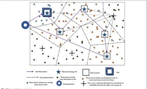
5.5 Mechanism of sink mobility in MBEENISH and iMBEENISH

This subsection clarifies the mechanism of sink mobility which is used in our proposed scheme. Figure 3 shows the

sink mobility mechanism of MBEENISH and iMBEENISH in a round. In every round, the mobile sink has to start its journey fromρ, and step by step sojourn at five minimum energy CHs in the network and then the mobile sink has to return back toρ. This movement of the sink fromρto a CH inside the network area and from CH toρis depicted in Eqs. (26d) and (26e) of the MSM, respectively. This is the tour of mobile sink in a single round. The mobile sink checks for the minimum distant sink location to its cur-rent location and then goes to that sink location which is at a shortest distance. The mobile sink moves fromρ to that minimum energy CH which is at the shortest distance fromρ. As the sink locations are predefined in a particu-lar round, after gathering data from that CH and nodes of that cluster, the mobile sink moves to the next sink loca-tion which is at the shortest distance. MS is staying on the minimum energy CH for gathering data and minimizes its load. Being part of the same network, if a CH dies, the sys-tem can become unstable. Nodes in blue color represent the cluster where the energy of CH in minimum, they send their data to the mobile sink directly instead of sending it to their CH to save their energy as depicted in Eq. (26a) of the MSM. Orange colored nodes are sensing the parame-ters but they are not sending the data to anyone because the sink has to pass through their cluster. So, these nodes keep queuing the data in their buffers until the mobile sink reaches their cluster. In Fig. 3, nodes in the green color sense the parameters; however, instead of sending

(13)

data directly to the mobile sink, they send the data to their respective CH for minimizing energy consumption. The CH, after receiving data from these nodes, aggregates and sends the data to the shortest distant sink location.

To elaborate the working of iMBEENISH, we present the whole scheme into three modules. The first mod-ule in Fig. 4 shows finding of normal, advanced, super, and ultra-super nodes. In the second module, shown in Fig. 5, clusters are formed. The CHs’ selection technique in our protocol is totally based upon probabilities which are assigned to each node on the basis of their residual energies. After clustering, the association of nodes with CHs takes place and clusters are formed. In the third mod-ule, Fig. 6 represents the data transmission from nodes and CHs, where every node checks whether to transmit its data to its corresponding CH or directly to the mobile sink. After that, CHs aggregate and send the data to the mobile sink, when the mobile sink comes to the most feasible closest location. In this procedure, sink mobility enables the nodes and CHs to transmit their data with minimum energy consumption.

6 Simulation results

In this section, we assess the performance of BEENISH, iBEENISH, MBEENISH, and iMBEENISH protocols using MATLAB. The assessment is done by considering the sta-bility period, network lifetime and packets sent to the BS, and packets received at the BS as performance parame-ters. The stability period is defined as the time interval from the start of the network till the death of the first node, whereas the instability period is the period from

Fig. 4Module 1: finding normal, advanced, super, and ultra-super nodes

Fig. 5Module 2: cluster formation and selection of CHs

the death of the first node till the death of the last node. Network lifetime is the time period until the last node dies. Data packets sent to the BS is the measure of the number of packets that are sent by nodes to the BS throughout the network lifetime.

We consider a WSN where 100 nodes are randomly deployed in the 10 m × 100 m network field. We are not considering energy loss due to signal collisions and

(14)

interference between signals of different nodes that are due to dynamic random channel conditions. Table 2 rep-resents the radio parameters we used in the proposed scheme simulations. We compare the proposed schemes (variants of BEENISH) with DEEC, DDEEC, and EDEEC.

For simulations, we consider the network that contains 40 normal nodes having E0 initial energy, whereas 30

advanced nodes (m=0.6 fraction of normal nodes) with 2 times more energy (a=2.0) than normal nodes. The 21 super nodes (m0=0.5 fraction of normal nodes)

contain-ingb=2.5 times more energy than normal nodes. Finally, 9 ultra-super nodes (m1 =0.3 fraction of normal nodes)

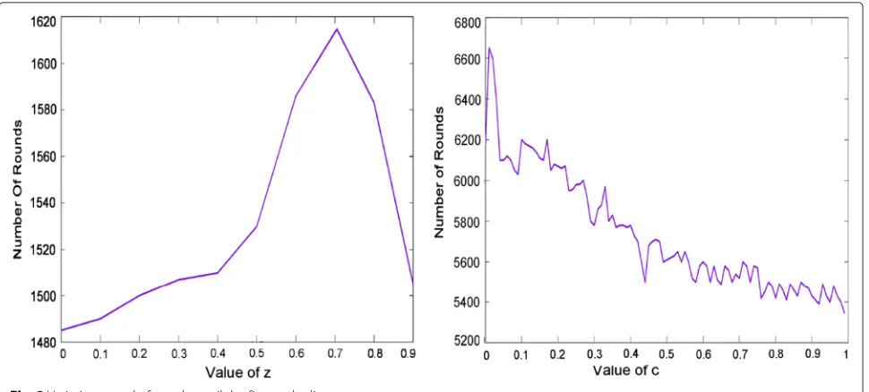
containingu = 3 times more energy than normal nodes. All nodes remain alive until their energy is consumed. Figure 7 shows alive nodes against the number of rounds. First node of DEEC, DDEEC, EDEEC, BEENISH, iBEEN-ISH, MBEENiBEEN-ISH, and iMBEENISH dies at 1287, 1523, 1595, 1754, 2046, 2237, and 2421 rounds, respectively, and all nodes die at 6520, 5144, 8046, 8109, 8521, 8630, and 9102 rounds, respectively. Figure 7 shows that alive nodes in BEENISH and iBEENISH gradually die which means that these two protocols are more efficient protocols than DEEC, EDEEC, and DDEEC. Nodes die in the follow-ing sequence: normal, advanced, super, and ultra-super. When a, b, u, m, m0, and m1 are changed, the

result-ing network lifetime, stability period, and behavior of the network also change. BEENISH and iBEENISH are per-forming much better than the other protocols because the threshold we set for the probability of nodes extend the network lifetime and stability period as shown in Fig. 7. From this figure, the stable period of MBEENISH is 92 % of the stable period of iMBEENISH. Similarly, the stable period of iBEENISH is 85 % of that of iMBEENISH. In the same way, BEENISH is 74 % of iMBEENISH in terms of stability period. DEEC, DDEEC, and EDEEC are 54, 63, and 66 % of iMBEENISH protocol in terms of sta-bility period. Figure 7b, c shows that with the variation in the dimensions of network from 100 m ×100 m to 250 m×250 m and 500 m×500 m, with varying number of nodes from 100 to 250 and 500, respectively; the network becomes sparse and nodes consume more energy during network establishment and transmissions.

Sink mobility prolongs the network lifetime and stabil-ity period to a greater extent as shown in Fig. 7. The sink moves from one location to the other and sojourns for a certain time making virtual sojourn regions. The mobile sink collects data from CHs and nodes which are lying in its current virtual sojourn region, and then moves to a next location and collects data from nodes and CHs of that sojourn region. The stability period of iMBEENISH is approximately 2350 rounds greater than iBEENISH and the stability period of MBEENISH is almost 2000 rounds more as compared to BEENISH. If we do not apply clus-tering in the network then these protocols will improve

0 2000 4000 6000 8000 10000 0

No. of Alive Nodes

Nodes alive during rounds

DEEC

(a)

Alive nodes for network dimensions 100m×100m with 100 nodes

0 2000 4000 6000 8000 10000 0

No. of Alive Nodes

DEEC

(b)

0 2000 4000 6000 8000 10000 0

No. of Alive Nodes

DEEC

(c)

Fig. 7 a–cAlive nodes during network lifetime

(15)

collect data from CHs and nodes. This results in effi-cient consumption of energy. It is clearly seen from the results that MBEENISH and iMBEENISH are more effi-cient than the other selected protocols in terms of stability period, network lifetime, and packets sent to the BS even in the case of when the network contains more super and advanced nodes as compared to normal nodes.

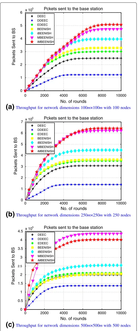
Figure 8 shows that MBEENISH and iMBEENISH send more number of packets to the BS as compared to the other selected protocols because every node checks the distance between its corresponding CH and the BS, and send packets to the BS if it is at a shorter distance. Pack-ets sent to the BS by nodes and CHs collectively make BEENISH, iBEENISH, MBEENISH, and iMBEENISH bet-ter than DEEC, DDEEC, and EDEEC. This is because DEEC, EDEEC, and DDEEC use clustering in such a way that the BS does not receive that much packets from non-CH nodes. But in iMBEENISH and MBEENISH, the sink goes near to the CHs and collects data. It also collects data from nodes which find it closer than their correspond-ing CHs. Accordcorrespond-ing to the sink mobility model (MSM), mobile sink sojourns at five sink locations in the net-work and gathers the data from those five CHs. Also, the sink collects data from every node which has any sink location in its communication range. Thus, this can lead to an increased number of packets sent to the BS. Throughput of the expanded network fields with extended number of nodes are shown in Fig. 8b, c. In Fig. 8b, the throughput of iMBEENISH and MBEENISH is almost the same. Figure 8c depicts that in initial rounds, iMBEENISH has higher throughput than MBEENISH; however, after that, MBEENISH has higher throughput because with 500 nodes in 500 m×500 m network dimensions it has a longer stability period.

Wireless links have slightly higher probability of bad link status, and there are chances that some of the pack-ets may drop on their way. So, Figs. 8 and 9 show that packets received are not the same as packets sent in every round using (random uniformed model for dropped pack-ets [30]). When nodes start to die, packpack-ets received at the BS also start to decrease; when all nodes are dead, throughput curve saturates (not increasing). In DEEC, the selected CHs vary with time. As a result, the number of received packets at the BS also vary. As shown in Fig. 9, the packets received are 30 % less than the packets sent to the BS which is shown in Fig. 8. Packets received for the networks with increased area (and more number of nodes as compared to the previous scenarios) are shown in Fig. 9b, c. The experimental results show that with an increase both in field dimensions and in number of nodes, throughput of the network increases. Also, the number of packets received by BS increases.

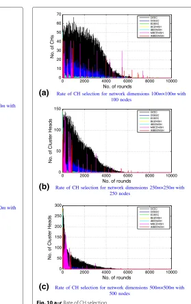
Figure 10 shows the rate at which CHs are selected in DEEC, EDEED, DDEEC, BEENISH, iBEENISH,

0 2000 4000 6000 8000 10000 0

Packets Sent to BS

Pckets sent to the base station

DEEC

(a)

Throughput for network dimensions 100m×100m with 100 nodes

0 2000 4000 6000 8000 10000 0

Packets Sent to BS

DEEC

(b)

0 2000 4000 6000 8000 10000 0

Packets Sent to BS

DEEC

(c)

Fig. 8 a–cThroughput of the network

(16)

0 2000 4000 6000 8000 10000 0

Packets Sent to BS

DEEC

(a)

Packets received at BS for network dimensions 100m×100m with 100 nodes

0 2000 4000 6000 8000 10000 0

Packets Received By BS

DEEC

(b)

0 2000 4000 6000 8000 10000 0

Packets Received By BS

DEEC

(c)

Fig. 9 a–cPackets received at BS

on random number and threshold value and this criteria does not guarantee optimum number of CHs. Due to this reason, surplus CHs are selected, which cause an early stage death of nodes in the respective protocols. Our proposed protocols also depend on a random number; however, we compensate this deficiency by adjusting the probability of CHs’ selection. In this way, the chances of CH selection tend toward its optimal value (as per our proposed protocols). Rate of CH selection decreases with new field dimensions and increased number of nodes, as obvious from Fig. 10b, c due to sparsity.

0 2000 4000 6000 8000 10000 0

(a)

Rate of CH selection for network dimensions 100m×100m with

100 nodes

0 2000 4000 6000 8000 10000 0

50 100 150

No. of rounds

No. of Cluster Heads

DEEC

(b)

250 nodes

0 2000 4000 6000 8000 10000 0

No. of Cluster Heads

DEEC

(c)

500 nodes

Fig. 10 a–cRate of CH selection

6.1 Performance trade-offs: which parameters routing schemes achieve on the cost of which ones

(17)

longer stability periods, enhanced network lifetime, and increased number of messages sent to the BS as com-pared to DEEC, DDEEC, and EDEEC, respectively. The sink mobility versions of the proposed BEENISH and iBEENISH perform better than the non-sink mobility ver-sions in terms of the selected performance evaluation parameters.

Sink mobility extends the network lifetime and stabil-ity period to a greater extent. The sink moves from one location to the other and sojourns for a certain time mak-ing virtual sojourn regions. The mobile sink collects data from CHs and nodes which are lying in its current vir-tual sojourn region, and then moves to a next location and collects data from nodes and CHs of that sojourn region.

Table 3Performance trade-offs made by the routing protocols being analyzed

Protocol Achievement Reference Price to pay Reference

iMBEENISH More alive nodes Fig. 7 Rate of CH selection Figs. 5 and 10

Packets sent to BS Fig. 8 Distance computation between CH and BS

Fig. 4

Packets received at BS Fig. 9 Sink movement to the CHs Fig. 6

Rate of CH selection Fig. 10 Energy consumption

MBEENISH More alive nodes Fig. 7 Sharp energy depletion

Packets sent to BS Fig. 8 Distance computation between CH and BS

Fig. 4

Packets received at BS Fig. 9 Sink movement to the CHs Fig. 3

Rate of CH selection Fig. 10 Lower stability period Fig. 1

iBEENISH More alive nodes Fig. 7 Sharp energy depletion

Packets sent to BS Fig. 8 Changes CH selection probability dynamically

Fig. 10

Packets received at BS Fig. 9 CH selection of high-energy nodes

Fig. 10

Rate of CH selection Fig. 10 Redundant transmission

BEENISH More alive nodes Fig. 7 Sharp energy depletion due to

four types of nodes

Fig. 1

Packets sent to BS Fig. 8 Rate of CH selection Fig. 10

Packets received at BS Fig. 9 Rate of CH selection Fig. 10

Rate of CH selection Fig. 10 Sudden energy depletion

EDEEC More alive nodes Fig. 7 Energy consumption due to three

nodes forwarding

Packets sent to BS Fig. 8 Throughput decreases due to packets loss in the midway

Fig. 9

Packets received at BS Fig. 9 Distant propagations Fig. 5

Rate of CH selection Fig. 10 More complexity involved

DDEEC More alive nodes Fig. 7 Energy consumption due to two

nodes forwarding

Packets sent to BS Fig. 8 As rounds pass, advanced nodes will have the same CH selection probability like that of the normal ones

Fig. 10

Packets received at BS Fig. 9 CH selection Fig. 10

Rate of CH selection Fig. 10 Redundant transmission and lower stability period

Fig. 7

DEEC More alive nodes Fig. 7 Overhead and complexity of

forming clusters

Fig. 10

Packets sent to BS Fig. 8 Less alive nodes Fig. 7

Packets received at BS Fig. 9 Less alive nodes Fig. 7

(18)

The stability period of iMBEENISH is approximately 2350 rounds greater than iBEENISH and the stability period of MBEENISH is almost 2000 rounds more as compared to BEENISH. If clustering is not applied to the network, then these protocols will improve effectively. This is because the sink mobility along with clustering is a difficult task to handle. MBEENISH and iMBEENISH are more energy efficient as compared to DEEC, DDEEC, and EDEEC as shown in Fig. 5 (Table 3). This is because the mobile sink goes to five sink locations to collect data from CHs and nodes. This results in more consumption of energy.

7 Conclusions

BEENISH considers the network with four different energy levels of nodes and selects CHs on the bases of residual energy of nodes and average energy of the net-work. So, in the BEENISH protocol, nodes with high energy are frequently selected as CHs as compared to low energy nodes. iBEENISH dynamically changes the CH selection probabilities of high energy nodes when their energy decreases. BEENISH and iBEENISH show better performance as compared to DEEC, DDEEC, and EDEEC, respectively, whereas iBEENISH shows better results than BEENISH in terms of network lifetime and through-put. Moreover, the implementation of the proposed sink mobility model facilitates the desired objectives. That is why MBEENISH and iMBEENISH perform better than BEENISH and iBEENISH in terms of the selected perfor-mance parameters.

Competing interests

The authors declare that they have no competing interests.

Acknowledgments

The authors would like to extend their sincere appreciation to the Deanship of Scientific Research at King Saud University for funding this research through Research Group Project No. RG#1435-051.

Author details

1_{COMSATS Institute of Information Technology, Islamabad, Pakistan.}2_College of CIS, King Saud University, Almuzahmiah, Saudi Arabia.3_{Department of} Electrical and Computer Engineering, University of Idaho, Moscow, USA.

Received: 15 November 2015 Accepted: 4 February 2016

References

1. VN Talooki, J Rodriguez, H Marques, Energy efficient and load balanced routing for wireless multihop network applications. Int. J. Distributed Sensor Netw.2014(13), article ID 927659 (2014). doi:10.1155/2014/927659 2. MA Hamid, MM Alam, MS Islam, CS Hong, S Lee, Fair data collection in

wireless sensor networks: analysis and protocol. Ann. Telecommun. 65(7–8), 433–446 (2010)

3. MA Mahmood, WK G Seah, I Welch, Reliability in wireless sensor networks: a survey and challenges ahead. Comput. Netw. Elsevier.79, 166–187 (2015)

4. O Zytoune, M El-Aroussi, Aboutajdine D, An energy efficient clustering protocol for routing in wireless sensor network. Int. J. Ad Hoc Ubiquitous Comput.7(1), 54–59 (2011)

5. C Ma, N Liu, Y Ruan, A dynamic and energy-efficient clustering algorithm in large-scale mobile sensor networks. Int. J. Distributed Sensor Netw. 2013, 8 article ID, 909243 (2013). doi:10.1155/2013/909243

6. A Ahmad, N Javaid, ZA Khan, U Qasim, T Alghamdi,(ACH)2_{: Routing}

scheme to maximize lifetime and throughput of wireless sensor networks. Sensors J. IEEE.14(10), 3516–3532 (2014). doi:10.1109/JSEN.2014.2328613 7. JM Kim, HS Seo, J Kwak, Routing protocol for heterogeneous hierarchical

wireless multimedia sensor networks. Wireless Pers. Commun.60(3), 559–569 (2011). doi:10.1007/s11277–011-0309-4

8. CB Abbas, R González, N Cardenas, G Villalba LJ, A proposal of a wireless sensor network routing protocol. Wireless Personal Commun.245, 410–422 (2007). doi:10.1007/978-0-387-74159-8_41

9. WR Heinzelman, A Chandrakasan, H Balakrishnan, inSystem Sciences, Proceedings of the 33rd Annual Hawaii International Conference on, vol. 2, iss. 4–7. Energy-efficient communication protocol for wireless microsensor networks, (2000), p. 10. doi:10.1109/HICSS.2000.926982

10. O Younis, F Sonia, HEED: a hybrid, energy-efficient, distributed clustering approach for ad hoc sensor networks. Mobile Comput IEEE Trans.3(4), 366–379 (2004). doi:10.1109/TMC.2004.41

11. G Smaragdakis, I Matta, A Bestavros, inSecond International Workshop on Sensor and Actor Network Protocols and Applications (SANPA 2004). SEP: a Stable Election Protocol for clustered heterogeneous wireless sensor network, vol. 3, (2004)

12. L Qing, Q Zhu, M Wang, Design of a distributed energy-efficient clustering algorithm for heterogeneous wireless sensor network. ELSEVIER Comput. Commun.29, 2230–2237 (2006)

13. B Elbhiri, R Saadane, S El-Fkihi, D Aboutajdine, inI/V Communications and Mobile Network (ISVC), 5th International Symposium on. Developed Distributed Energy-Efficient Clustering (DDEEC) for heterogeneous wireless sensor networks, (2010), pp. 1–4. doi:10.1109/ISVC.2010.5656252 14. P Saini, AK Sharma, inParallel Distributed and Grid Computing (PDGC), 1st

International Conference on, iss. 28–30. E-DEEC—Enhanced Distributed Energy Efficient Clustering scheme for heterogeneous WSN, (2010), pp. 205–210. doi:10.1109/PDGC.2010.5679898

15. TN Qureshi, N Javaid, AH Khan, A Iqbal, E Akhtar, M Ishfaq, BEENISH: Balanced Energy Efficient Network Integrated Super Heterogeneous Protocol for Wireless Sensor Networks. Proc Comput. Sci.19, 920–925 (2013). ISSN 1877–0509. http://dx.doi.org/10.1016/j.procs.2013.06.126. Accessed 12 Feb 2016

16. MH Anisi, AH Abdullah, Y Coulibaly, SA Razak, EDR: efficient data routing in wireless sensor networks. Int. J. Ad Hoc Ubiquitous Comput. 12(1/2013), 46–55 (2013). doi:10.1504/IJAHUC.2013.051390 17. T Mikoshi, S Momma, T Takenaka, PARC: Power Aware Routing and

Clustering scheme for wireless sensor networks. IEICE Trans Commun. E94–B(12), 3471–3479 (2011)

18. D Seong, J Park, J Lee, M Yeo, J Yoo, Data gathering by mobile sinks with data-centric probe in sensor networks. IEICE Trans Commun.E94–B(7), 2133–2136 (2011)

19. H Chen, D Qian, W Wu, Practical distributed location service for wireless sensor networks with mobile sinks. IEICE Trans Commun.E95–B(9), 2838–2851 (2012)

20. E Lee, S Park, H Park, S-H Kim, Independent grid structure-based routing protocol in wireless sensor networks. IEICE Trans. Commun.E96–B(1), 309–312 (2013)

21. H Zhao, G Songtao, X Wang, F Wang, Energy-efficient topology control algorithm for maximizing network lifetime in wireless sensor networks with mobile sink. Appl. Soft Comput.34(2015), 539–550

22. F Tashtarian, M Hossein Yaghmaee Moghaddam, K Sohraby, S Effati, On maximizing the lifetime of wireless sensor networks in event-driven applications with mobile sinks. Vehicular Technology, IEEE Transactions. 64.7(2015), 3177–3189

23. J Luo, J-P Hubaux, Joint sink mobility and routing to maximize the lifetime of wireless sensor networks: the case of constrained mobility. Netw. IEEE/ACM Trans.18(3), 871–884 (2010). doi:10.1109/TNET.2009.2033472 24. M Imran, NA Zafar, MA Alnuem, MS Aksoy, A Vasilakos, Formal verification

and validation of a movement control actor relocation algorithm for wireless sensor and actor networks. Wireless Netw. J, 1–19 (2015). doi:10.1007/s11276-015-0962-8

25. N Haider, M Imran, M Younis, NM Saad, M Guizani, inProceedings of the 2015 IEEE International Conference on Communication (ICC). A novel mechanism to restore actor connected coverage in wireless sensor and actor networks. (UK, London, 2015), pp. 6383–6388

(19)

27. J Cota-Ruiz, J-G Rosiles, P Rivas-Perea, E Sifuentes, A distributed localization algorithm for wireless sensor networks based on the solutions of spatially-constrained local problems. Sensors J. IEEE.13(6), 2181–2191 (2013). doi:10.1109/JSEN.2013.2249660

28. AW Khan, AH Abdullah, MA Razzaque, JI Bangash, VGDRA: A Virtual Grid-Based Dynamic Routes Adjustment Scheme for mobile sink-based wireless sensor networks. Sensors J. IEEE.15(1), 526–534 (2015) 29. S Park, E Lee, M-S Jin, Kim S-H, Cluster-based communication for mobile

sink groups in large-scale wireless sensor networks Trans. IEICE Commun. E94–B(1), 307–310 (2011)

30. Q Zhou, X Cao, S Chen, G Lin, A solution to error and loss in wireless network transfer. Int. Conf. Wireless Netw. Inform. Syst.28–29, 312–315 (2009). doi:10.1109/WNIS.2009.103

Submit your manuscript to a

journal and beneﬁ t from:

7Convenient online submission

7Rigorous peer review

7Immediate publication on acceptance

7Open access: articles freely available online 7High visibility within the ﬁ eld

7Retaining the copyright to your article