A new two level implicit scheme of order two in time and four in space based on half step spline in compression approximations for unsteady 1D quasi linear biharmonic equations

R E S E A R C H

Open Access

A new two-level implicit scheme of order

two in time and four in space based on

half-step spline in compression

approximations for unsteady 1D quasi-linear

biharmonic equations

R.K. Mohanty

_{, Sachin Sharma}

_{and Swarn Singh}

*_{Correspondence:} [email protected]

1_{Department of Applied} Mathematics, South Asian University, New Delhi, India Full list of author information is available at the end of the article

Abstract

In this article, we discuss a new two-level implicit scheme of order of accuracy two in time and four in space based on the spline in compression approximations for the numerical solution of 1D unsteady quasi-linear biharmonic equations. We use only two half-step points and a central point on a uniform mesh for spline approximations and derivation of the method. The proposed method is derived directly from the continuity condition of the first order derivative of the spline function. For model linear problem, the proposed scheme is shown to be unconditionally stable. The proposed method has successfully tested on the Kuramoto–Sivashinsky equation and extended the Fisher–Kolmogorov equation. From the computational experiment, we obtain better numerical results compared to the results obtained by other

researchers.

MSC: 65M06; 65M12; 65M22; 65Y20

Keywords: Quasi-linear biharmonic equations; Spline in compression function; Kuramoto–Sivashinsky equation; Newton’s iterative method

1 Introduction

We consider the fourth order unsteady biharmonic equation with variable coefficient of the form

A(x,t)uxxxx+ut=f(x,t,u,ux,uxx,uxxx), (x,t)∈, (1.1)

where≡ {(x,t)|0 <x< 1,t> 0}is the solution space.

The equation above may be written in a coupled manner as follows:

uxx=v, (x,t)∈, (1.2)

A(x,t)vxx= –ut+f(x,t,u,ux,v,vx)≡g(x,t,u,v,ux,vx,ut), (x,t)∈. (1.3)

The initial and boundary values are given by

u(x, 0) =u0(x), 0≤x≤1, (1.4)

u(0,t) =a0(t), u(1,t) =a1(t), t> 0, (1.5)

uxx(0,t) =v(0,t) =b0(t), uxx(1,t) =v(1,t) =b1(t), t> 0, (1.6)

whereu0,a0,b0,a1, andb1are smooth functions, and we assume that their required higher

order derivatives exist in the solution region.

Many physical problems in terms of linear or nonlinear biharmonic equations are of common occurrence in engineering and science. Famous nonlinear PDEs of type (1.1) are generalized Kuramoto–Sivashinsky (GKS) equation, extended Fisher–Kolmogorov (EFK) equation, etc. The physical appearance and behavior of these equations were discussed in [1–10]. During the last decade, several numerical methods have been discussed for the solution of GKS and EFK equations. Xu and Shu [11] proposed a local discontinu-ous Galerkin method for the Kuramoto–Sivashinsky (KS) equation. Khater and Temsah [12] used a Chebyshev spectral collocation method to solve the GKS equation. Lai and Ma [13] studied a lattice Boltzmann method, and Uddin et al. [14] discussed a mesh-free method for the numerical solution of GKS equation. Using a B-spline collocation method, Mittal and Arora [15] and Lakestani and Dehghan [16] solved the GKS equation. Using a cubic Hermite collocation method, Ganaiea et al. [17] obtained the numerical solution of KS equation. Most recently, Mohanty and Kaur [18] developed a Numerov type com-pact variable mesh method for the solution of KS equation. A polynomial scaling function technique was used by Rashidinia and Jokar [19] for solving the GKS equation. Danum-jaya and Pani [20] constructed a numerical scheme based on an orthogonal cubic spline collocation method for the solution of EFK equation. Using a splitting technique, Doss and Nandini [21] proposed anH1-Galerkin mixed finite element method for the solution of EFK equation.

solution of nonlinear time-dependent biharmonic equation have been developed so far. In the present article, we propose a new two-level implicit numerical method of order of accuracy two in time and four in space, based on trigonometric spline approximations for the solution of PDE (1.1).

We use only two half-step points and one central point in x-direction at each time level, and no fictitious points are required for incorporating the boundary conditions. It is known that the difference methods for the biharmonic equation are based on five or more grid points inx-direction, and thus require fictitious points outside the solution region. These fictitious points are then eliminated by discretizing the given derivative boundary conditions. However, using the standard second order central differences for the bound-ary conditions, the accuracy of the overall numerical scheme is affected even if a higher order scheme is used at internal grid points. The algorithm presented in this paper reduces the fourth order PDE into coupled elliptic-parabolic equations, and we do not require to discretize the derivative boundary conditions. It attains order of accuracy two in time and four in space by using only three spatial grid points at each time level. The main attraction of this work is the application of the proposed high accuracy numerical method to the KS equation, GKS equation, and EFK equation.

The rest of this paper is organized as follows: In Sect.2, we discuss the spline in com-pression function and its properties for the coupled equation. In Sect.3, we present a new two-level implicit spline in compression method for 1D unsteady quasi-linear biharmonic problem of second kind, which is further derived in Sect.4. In Sect.5, the proposed spline in compression method is shown to be unconditionally stable for a linear biharmonic prob-lem. In Sect.6, we implement the proposed method on the KS equation, GKS equation, and EFK equation. We also compare our numerical results with the results of other re-searchers available in the literature. It is shown that the proposed numerical method yields better results as compared to the results given by other researchers. Concluding remarks are given in Sect.7.

2 Spline in compression approximations and their properties

For the approximate solution of the proposed initial-boundary value problem, we dis-cretize the space interval [0, 1] as 0 =x0<x1<· · ·<xL<xL+1= 1, where Lis a positive

integer. The proposed spline approximation consists of two half-step pointsxl±1/2and a

central pointxl,l= 0, 1, 2, . . . ,Lwith two end pointsx0 andxL+1. The neighboring

half-step points are defined asxl–1/2=xl–h₂ andxl+1/2=xl+h₂,l= 1(1)L, whereh=xl+1–xl, l= 0(1)Lis the mesh size inx-direction andk=tj+1–tj> 0,j= 0, 1, 2, . . . , is the mesh

spacing int-direction. LetU_lj=u(xl,tj) be the exact solution value ofu(x,t) approximated byuj_l. Also letV_lj=v(xl,tj) be the exact solution value ofv(x,t) approximated byvj_l. Now supposeM=UxxandN=Vxx.

A non-polynomial spline function which interpolates the value U_lj atjth time level is given by

Pj(x) =ajl+b j

l(x–xl) +cjlsin

τ(x–xl)

+dj_lcosτ(x–xl)

,

xl–1≤x≤xl,l= 1(1)L+ 1,j> 0, (2.1)

which satisfies the following properties atjth time level:

(ii) Pj(xl) =U_lj,Pj(xl–1) =Ulj–1,

whereτ is an arbitrary parameter andP_j(xl) =Mj_l,P_j(xl–1) =Mj_l–1,Pj(xl–1/2) =Mj_l–1/2.

Using these properties, we get the coefficients

aj_l=U_lj+M spline in compression functionPj(x) defined as

Pj(x) =

Similarly, a non-polynomial spline function which interpolates the valueV_ljatjth time level is given by

Qj(x) =

whereQj(x) satisfies the following properties atjth time level:

(i) Qj(x)∈C2[0, 1],

(ii) Qj(xl) =V_lj,Qj(xl–1) =Vlj–1, andQj(xl) =N j

Using the continuity of the first derivative ofPj(x) andQj(x), that is,P_j(xl–) =P_j(xl+) and

Q_j(xl–) =Q_j(xl+), we obtain the following consistency conditions:

U_lj₊₁– 2U_lj+U_lj_–1

h2 =αM

j

l+1/2+ 2βM

j l+αM

j l–1/2+O

h4, l= 1(1)L, (2.6)

V_lj₊₁– 2V_lj+V_lj_–1

h2 =αN

j

l+1/2+ 2βN

j l+αN

j l–1/2+O

h4, l= 1(1)L, (2.7) where

α= 1 2μ2

μ

sinμ–cosμ =

1 3–

μ2

90+O

μ4, (2.8)

β= 1

2μ2(1 –μcotμ) =

1 6+

μ2

90+O

μ4. (2.9)

On equating the coefficients ofMj_landN_ljin (2.7)–(2.8), we obtain the condition

α+β= 1/2. (2.10)

Substituting the values ofαandβin (2.10) and neglectingO(μ4_{) terms, we get}

tan(μ/2) =μ/2. (2.11) The above equation has an infinite number of roots, the smallest positive non-zero root being given byμ= 8.986818916.

Further, from (2.2)–(2.5), we get

P_j(xl–1/2) =

U_lj–U_lj_–1

h –

h

4

2βM_lj–αM_lj_–1/2, (2.12)

P_j(xl+1/2) =

U_lj₊₁–U_lj

h +

h

4

2βMj_l–αMj_l+1/2, (2.13)

Q_j(xl–1/2) =

V_lj–V_lj_–1

h –

h

4

2βN_lj–αN_lj_–1/2, (2.14)

Q_j(xl+1/2) =

V_lj₊₁–V_lj

h +

h

4

2βN_lj–αN_lj_+1/2. (2.15) Relations (2.12)–(2.15) are important properties of spline functions.

3 Formulation of a spline in compression method

In order to derive the high accuracy numerical method based on a spline function and its properties for PDEs (1.2)–(1.3), we require the following three point approximations:

Forr= 0,±1, we denote

¯

tj=tj+θk, (3.1)

¯

Aj_l=A(xl,¯tj), (3.2)

¯

¯

Further, we define the following approximations:

¯

From the properties of spline functions (2.12)–(2.15), we have the following approxima-tions:

We consider the following linear combinations in order to increase the accuracy of the scheme:

4 Derivation of the numerical algorithm

In this section, we derive the spline method from the consistency conditions given by (2.6)–(2.7).

F_lj_+1/2+F_lj_–1/2= 2F_lj+Oh2= 2(A00V20+U01) +O

Simplifying approximations (3.5)–(3.18) using a Taylor series expansion, we obtain

With the help of (4.11)–(4.23), from (3.19)–(3.21), we obtain Further, we can write

1

Simplifying (3.37)–(3.38), we obtain

ˆ Now, using the above approximations and simplifying (3.32)–(3.35), we obtain

Equating the coefficient ofh2_{to zero in Eqs. (4.41) and (4.42), we obtainc=d=}–1 It is easy to verify that

10U¯_tlj +

Comparing (4.59)–(4.60) with the consistency conditions (4.9)–(4.10), we obtain

ˆ solve the quasi-linear differential equation when A=A(x,t,u), we need to modify the method (3.39)–(3.40). The details of the technique to write numerical schemes for quasi-linear problems are discussed in [18,23,26,28]. The same technique can be used here to write a numerical scheme for quasi-linear differential equation (1.1) whenA=A(x,t,u).

5 Stability analysis

For stability analysis of the proposed method, we consider the linearized KS equation with-out second order derivative term

whereγ,δ> 0 are constants. Applying the proposed method (3.39)–(3.40) to the linearized KS equation (5.1) and neglecting local truncation errors, we obtain the following non-polynomial schemes in a coupled form:

12uj_l+1_–1– 2u_lj+1+uj_l+1₊₁–h2vj_l+1_–1+ 10v_lj+1+vj_l+1₊₁

To apply the von Neumann linear stability method, we consider that the numerical so-lutions are given byuj_l=ρj_eiηl_andvj

l=σjeiηlfori= √

–1, whereρ,σ are amplification factors andηis the phase angle. Substituting these in Schemes (5.2)–(5.3), we obtain the following matrix form: Now, define the amplification matrixHas

H=A–1B. (5.5)

Let the eigenvalues of the amplification matrixHbeω=ω1,ω2. The von Neumann

nec-essary condition for linear stability of system (5.2)–(5.3) is thatmax|ω| ≤1. By direct cal-culation, the eigenvalues ofHare given by

C∗= –h

2

4

1 –1 3sin

2η

2

2

–δλ 2 sin

4η

2,

D=γ λh 8

1 –1 3sin

2η

2

+γ αλh

3

48 sin

2η

2sinη. It is noticed thatmax|ω1|= 1 andmax|ω2| ≤1 if

δλ

2 h

2

1 –1 3sin

2η

2

2 sin4η

2≥0. (5.6)

Inequality (5.6) is true for all values of phase angleη. Hence system (5.3)–(5.4) is uncon-ditionally stable.

6 Numerical results

In this section, we apply the proposed spline in compression method to the GKS equa-tion, KS equaequa-tion, and EFK equation with different parameters. The exact solutions are provided as a test procedure. The initial and boundary conditions can be obtained from the exact solutions. Whenever PDE (1.1) is quasi-linear or nonlinear, the proposed method builds a coupled nonlinear block system. In the following examples, we use Newton’s block Gauss–Seidel iteration method [30–33] for the solution of a coupled nonlinear block sys-tem. In each case iterations were stopped when the absolute error tolerance ≤10–10_is

achieved.

Example1 (Kuramoto–Sivashinsky equation)

ut+uux+uxx+uxxxx= 0, –30 <x< 30,t> 0. (6.1)

The exact solution [13,34] is given by

u(x,t) =β0+

15 19

11 19

–9tanhκ(x–β0t–x0)

+ 11tanh3κ(x–β0t–x0)

.

For computation, we choose the valuesβ0= 5,κ=1₂

11

19,x0= –12 in the solution domain

[–30, 30] withh= 1/150 andk= 1/100. To check the accuracy of the proposed method, we compute the global relative errors (GRE) defined using the formula

GRE =

L l=1|u

j l–U

j l|

L l=1|U

j l|

,

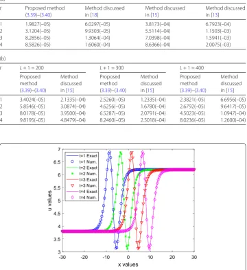
whereuj_landU_ljdenote the numerical and exact solution values at the grid point (xl,tj), respectively. We compare our numerical results with the results given in [13,15,18]. The GREs for the solutions of (6.1) are presented in Table1a at different time levels. We show the comparison of exact and numerical solutions at various time levels in Fig.1. In Ta-ble1b, the GRE is compared with the results given in [15] to exhibit the effect of change in the number of grid points.

Example2 (Kuramoto–Sivashinsky equation)

Table 1 Example1: The global relative errors

(a)

t Proposed method (3.39)–(3.40)

Method discussed in [18]

Method discussed in [15]

Method discussed in [13]

1 1.9827(–05) 6.0297(–05) 3.8173(–04) 6.7923(–04)

2 3.1204(–05) 9.9303(–05) 5.5114(–04) 1.1503(–03)

3 8.2856(–05) 1.3064(–04) 7.0398(–04) 1.5941(–03)

4 8.5826(–05) 1.6060(–04) 8.6366(–04) 2.0075(–03)

(b)

t L+ 1 = 200 L+ 1 = 300 L+ 1 = 400

Proposed method (3.39)–(3.40)

Method discussed in [15]

Proposed method (3.39)–(3.40)

Method discussed in [15]

Proposed method (3.39)–(3.40)

Method discussed in [15]

1 3.4024(–05) 2.1335(–04) 2.5260(–05) 1.2335(–04) 2.3821(–05) 6.6956(–05) 2 5.8546(–05) 3.0874(–04) 4.6256(–05) 1.6780(–04) 2.6792(–05) 9.6417(–05) 3 8.0178(–05) 3.9500(–04) 6.5287(–05) 2.0791(–04) 4.5023(–05) 1.0947(–04) 4 9.8195(–05) 4.8479(–04) 8.2460(–05) 2.5018(–04) 8.0236(–05) 1.2600(–04)

Figure 1Example1: Comparison between numerical and exact solutions at different time levels

The exact solution [13,34] is given by

u(x,t) =β0+

15 19√19

–3tanhκ(x–β0t–x0)

+tanh3κ(x–β0t–x0)

.

For computation, we choose the valuesβ0= 5,κ=₂√1₁₉,x0= –25 in the interval [–50, 50]

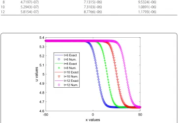
withh= 1/200 andk= 1/100. In Table2, the GRE is compared with the results given in [13,

15]. At various time levels, we present the graph between numerical and exact solutions in Fig.2.

Example3 (Generalized Kuramoto–Sivashinsky equation)

Table 2 Example2: The global relative errors

t Proposed method (3.39)–(3.40) Method discussed in [15] Method discussed in [13]

6 3.9866(–07) 6.5093(–06) 7.8808(–06)

8 4.7197(–07) 7.1315(–06) 9.5324(–06)

10 5.2943(–07) 7.3103(–06) 1.0891(–06)

12 5.8154(–07) 8.7766(–06) 1.1793(–06)

Figure 2Example2: Comparison between numerical and exact solutions at different time levels

Table 3 Example3: The global relative errors

t Proposed method (3.39)–(3.40) Method discussed in [18] Method discussed in [13]

1 1.1734(–05) 8.4059(–05) 2.5945(–02)

2 3.9568(–05) 2.7154(–04) 2.7959(–02)

3 7.8924(–05) 5.3351(–04) 2.6701(–02)

4 1.2925(–04) 8.5210(–04) 3.5172(–02)

The exact solution [13,34] is given by

u(x,t) =β0+ 9 – 15

tanhκ(x–β0t–x0)

+tanh2κ(x–β0t–x0)

–tanh3κ(x–β0t–x0)

.

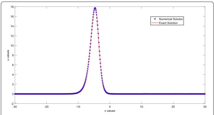
For computation, we choose the valuesβ0= 6,κ= 0.5,x0= –10 in the solution domain

[–30, 30] withh= 1/10 andk= 1/10,000. The GRE is reported in Table3and the results are compared with the results given in [13,18]. In Fig.3, we present the comparison of exact and numerical solutions att= 1.

Example4 (Extended Fisher–Kolmogorov equation)

Figure 3Example3: Comparison between numerical and exact solutions att= 1

The initial and boundary conditions [20] are given by

u(x, 0) = –sin(πx), –4≤x≤4,

u(–4,t) = 0, u(4,t) = 0, t> 0,

uxx(–4,t) = 0, uxx(4,t) = 0.

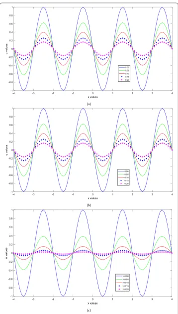
For the above conditions, we plotted graphs (Fig.4a–4c) of the computed solution at dif-ferent time levels. We observe that the behavior of the numerical solution atγ = 0 and

γ = 0.0001 is almost similar. However, we notice that as timet increases, the solution curves fall to zero rapidly forγ = 0.1, which ensures the stabilizing character of the EFK equation.

7 Final discussion

In this paper, we have discussed a new two-level implicit numerical method in a coupled form based on spline in compression approximations for the solution of time-dependent quasi-linear biharmonic equations. The proposed spline method uses only three spatial grid pointsxl,xl±1/2, and no fictitious points for incorporating the boundary conditions

(a)

(b)

(c)

Figure 4Example4: (a) The profiles ofu(x,t) versusxforγ= 0. (b) The profiles ofu(x,t) versusxfor

Acknowledgements

The authors thank the reviewers for their valuable suggestions, which substantially improved the standard of the paper.

Funding

This research work is supported by CSIR-SRF, Grant No: 09/045(1161)/2012-EMR-I.

Competing interests

The authors declare that they have no competing interests.

Authors’ contributions

All authors drafted the manuscript, and they read and approved the final version.

Author details

1_{Department of Applied Mathematics, South Asian University, New Delhi, India.}2_{Department of Mathematics, Faculty of}

Mathematical Sciences, University of Delhi, Delhi, India. 3_{Department of Mathematics, Sri Venkateswara College,}

University of Delhi, New Delhi, India.

Publisher’s Note

Springer Nature remains neutral with regard to jurisdictional claims in published maps and institutional affiliations.

Received: 3 August 2018 Accepted: 9 October 2018

References

1. Aronson, D.G., Weinberger, H.F.: Multidimensional nonlinear diffusion arising in population genetics. Adv. Math.30, 33–67 (1978)

2. Conte, R.: Exact solutions of nonlinear partial differential equations by singularity analysis. In: Lecture Notes in Physics, pp. 1–83. Springer, Berlin (2003)

3. Dee, G.T., van Saarloos, W.: Bistable systems with propagating fronts leading to pattern formation. Phys. Rev. Lett.60, 2641–2644 (1988)

4. Hooper, A.P., Grimshaw, R.: Nonlinear instability at the interface between two viscous fluids. Phys. Fluids28, 37–45 (1985)

5. Hornreich, R.M., Luban, M., Shtrikman, S.: Critical behaviour at the onset ofk-space instability at theλline. Phys. Rev. Lett.35, 1678–1681 (1975)

6. Kuramoto, Y., Tsuzuki, T.: Persistent propagation of concentration waves in dissipative media far from thermal equilibrium. Prog. Theor. Phys.55, 356–369 (1976)

7. Saprykin, S., Demekhin, E.A., Kalliadasis, S.: Two-dimensional wave dynamics in thin films. I. Stationary solitary pulses. Phys. Fluids17, 117105 (2005)

8. Sivashinsky, G.I.: Instabilities, pattern-formation, and turbulence in flames. Annu. Rev. Fluid Mech.15, 179–199 (1983) 9. Tatsumi, T.: Irregularity, regularity and singularity of turbulence. In: Turbulence and Chaotic Phenomena in Fluids.

Iutam, pp. 1–10 (1984)

10. Zhu, G.: Experiments on director waves in nematic liquid crystals. Phys. Rev. Lett.49, 1332–1335 (1982) 11. Xu, Y., Shu, C.W.: Local discontinuous Galerkin methods for the Kuramoto–Sivashinsky equations and the Ito-type

coupled KdV equations. Comput. Methods Appl. Mech. Eng.195, 3430–3447 (2006)

12. Khater, A.H., Temsah, R.S.: Numerical solutions of the generalized Kuramoto–Sivashinsky equation by Chebyshev spectral collocation methods. Comput. Math. Appl.56, 1456–1472 (2008)

13. Lai, H., Ma, C.: Lattice Boltzmann method for the generalized Kuramoto–Sivashinsky equation. Physica A388, 1405–1412 (2009)

14. Uddin, M., Haq, S., Siraj-ul-Islam: A mesh-free numerical method for solution of the family of Kuramoto–Sivashinsky equations. Appl. Math. Comput.212, 458–469 (2009)

15. Mittal, R.C., Arora, G.: Quintic B-spline collocation method for numerical solution of the Kuramoto–Sivashinsky equation. Commun. Nonlinear Sci. Numer. Simul.15, 2798–2808 (2010)

16. Lakestani, M., Dehghan, M.: Numerical solutions of the generalized Kuramoto–Sivashinsky equation using B-spline functions. Appl. Math. Model.36, 605–617 (2012)

17. Ganaiea, I.A., Arora, S., Kukreja, V.K.: Cubic Hermite collocation solution of Kuramoto–Sivashinsky equation. Int. J. Comput. Math.93, 223–235 (2016)

18. Mohanty, R.K., Kaur, D.: Numerov type variable mesh approximations for 1D unsteady quasi-linear biharmonic problem: application to Kuramoto–Sivashinsky equation. Numer. Algorithms74, 427–459 (2017)

19. Rashidinia, J., Jokar, M.: Polynomial scaling functions for numerical solution of generalized Kuramoto–Sivashinsky equation. Appl. Anal.96, 293–306 (2017)

20. Danumjaya, P., Pani, A.K.: Orthogonal cubic spline collocation method for the extended Fisher–Kolmogorov equation. J. Comput. Appl. Math.174, 101–117 (2005)

21. Doss, L.J.T., Nandini, A.P.: AnH1_{-Galerkin mixed finite element method for the extended Fisher–Kolmogorov equation.}

Int. J. Numer. Anal. Model. Ser. B3, 460–485 (2012)

22. Stephenson, J.W.: Single cell discretizations of order two and four for biharmonic problems. J. Comput. Phys.55, 65–80 (1984)

23. Mohanty, R.K.: An accurate three spatial grid-point discretization ofO(k2_+h4_{) for the numerical solution of one-space}

dimensional unsteady quasi-linear biharmonic problem of second kind. Appl. Math. Comput.140, 1–14 (2003) 24. Jain, M.K., Iyenger, S.R.K., Pillai, A.C.R.: Difference schemes based on spline in compression for the solution of

conservative laws. Comput. Methods Appl. Mech. Eng.38, 137–151 (1983)

26. Mohanty, R.K., Gopal, V.: High accuracy non-polynomial spline in compression method for one-space dimensional quasilinear hyperbolic equations with significant first order space derivative term. Appl. Math. Comput.238, 250–265 (2014)

27. Talwar, J., Mohanty, R.K., Singh, S.: A new spline in compression approximation for one space dimensional quasilinear parabolic equations on a variable mesh. Appl. Math. Comput.260, 82–96 (2015)

28. Mohanty, R.K., Sharma, S.: High accuracy quasi-variable mesh method for the system of 1D quasi-linear parabolic partial differential equations based on off-step spline in compression approximations. Adv. Differ. Equ.2017, 212 (2017)

29. Mohanty, R.K., Sharma, S.: A new two-level implicit scheme for the system of 1D quasi-linear parabolic partial differential equations using spline in compression approximations. Differ. Equ. Dyn. Syst. (2018).

https://doi.org/10.1007/s12591-018-0427-5

30. Jain, M.K., Jain, R.K., Mohanty, R.K.: Fourth order difference method for the one-dimensional general quasi-linear parabolic partial differential equation. Numer. Methods Partial Differ. Equ.6, 311–319 (1990)

31. Jain, M.K., Jain, R.K., Mohanty, R.K.: High order difference methods for system of 1D non-linear parabolic partial differential equations. Int. J. Comput. Math.37, 105–112 (1990)

32. Mohanty, R.K., Jha, N., Evans, D.J.: Spline in compression method for the numerical solution of singularly perturbed two point singular boundary value problems. Int. J. Comput. Math.81, 615–627 (2004)

33. Mohanty, R.K., Jha, N.: A class of variable mesh spline in compression methods for singularly perturbed two point singular boundary value problems. Appl. Math. Comput.168, 704–716 (2005)