R E S E A R C H
Open Access
Optimizing the performance of non-fading
and fading networks using CSMA with joint
transmitter and receiver sensing
Mariam Kaynia
*and Geir E Øien
Abstract
We consider a mobile ad hoc network where packets belonging to specific transmitters arrive randomly in space and time according to a 3-D Poisson point process, and are upon arrival transmitted to their intended destinations using the carrier sensing multiple access (CSMA) MAC protocol. A packet transmission is considered successful if the received SINR is above a predefined threshold for the duration of the packet. A simple fully-distributed joint transmitter-receiver sensing scheme is proposed for the CSMA protocol to improve its performance in both
non-fading and fading networks. The outage probability of this enhanced version of CSMA is derived and optimized with respect to the sensing thresholds. In order to derive a mathematical expression for the optimal sensing thresholds, the inherent hidden and exposed node problems of CSMA are considered and efficiently balanced. The performance of this improved CSMA protocol is compared to the other flavors of CSMA, and shown to bring about significant performance gain.
1 Introduction
Medium access control (MAC) layer design is com-monly applied to address the problem of allocating scarce resources in a wireless network. Various MAC protocols are proposed in order to share the communication chan-nel in the most efficient manner, in order to minimize the destructive interference. One such protocol that has gained great popularity is carrier sensing multiple access (CSMA). This protocol is successfully employed in the IEEE 802.11 standard family, and many enhancements have been proposed and implemented in order to min-imize the inherent hidden and exposed node problems [1-3]. Nevertheless, there is still room for improvement, in particular in networks with high density of simultaneous transmissions. This provides the motivation behind our study.
Numerous studies have evaluated the performance of the CSMA protocol, evaluating its performance in terms of throughput and bit error rate [4-6]. Much of this study confirms CSMA’s superiority over other protocols, such as ALOHA, with natural tradeoffs in other domains such
*Correspondence: mariam.kaynia@iet.ntnu.no
Department of Electronics and Telecommunications, Norwegian University of Science and Technology, 7491 Trondheim, Norway
as transmission rate and delay [1,6]. Also, many exten-sions have been proposed to improve the performance of CSMA [7-9]. However, the conventional model used in most of these studies assumes that the topology of the network is known, and that multiple links cannot commu-nicate simultaneously. Such assumptions are not realistic for mobile ad hoc networks (MANETs). The closest model to a real-life ad hoc network is that used in [10,11], where users are assumed to be Poisson distributed in space and each transmitter communicates with its own receiver using ALOHA, while allowing for simultaneous commu-nication between links. This model was embraced in [12], and is also applied in our study.
Choosing the right value for CSMA’s sensing thresh-old (which the backoff decision is based on) is of great importance for the performance of this protocol. Many studies have proposed various adaptation schemes to find the optimal carrier sensing threshold of CSMA to enhance the throughput and the transmission reliability in dynam-ically changing networks [13-15]. In [2], a novel analytical model was introduced for determining the optimal car-rier sensing range in ad hoc networks by minimizing the sum of the hidden and exposed terminal areas. The optimization is done in terms of aggregate throughput,
yielding that the optimal carrier sensing range is approx-imately equal to the interference range. The study of [16] further improves the carrier sensing capability of CSMA by adding fairness to the equation, while retaining the throughput performance. The shortcoming of this study is that only six node pairs are considered in the perfor-mance evaluation, limiting the applicability of the results to a randomly distributed ad hoc network with high den-sity of simultaneous transmissions. Moreover, it is shown in [7] that the optimal algorithm is for the senders to keep the product of their transmit power and carrier sensing threshold equal to a constant. However, this algo-rithm is not distributed, and is dependent on the estima-tion of signal powers. Another algorithm for maximizing the throughput is to decrease the sensing range as long as the network remains sufficiently connected [17]. An improved carrier sensing threshold adaptation algorithm was proposed in [8], where each node chooses the sens-ing threshold that maximizes the number of successful transmissions in its neighborhood. The drawback of this technique is that it relies on the collection of information over a period of time, which entails higher complexity, and introduces delays. Zhu et al. derive in [9] the optimal sensing threshold of the conventional CSMA protocol to beβt = ρ(1+β1/α)α, whereρ represents the transmit-ted signal strength,α is the path loss exponent, andβ is the minimum required signal-to-interference-plus-noise ratio (SINR) threshold for correct reception of packets. The optimized CSMA protocol was evaluated on a real test-bed in [18].
In [12], a new version of the CSMA protocol is pro-posed, denoted CSMARX, where the receiver (as opposed
to the transmitter in CSMATX) performs the channel
sensing and makes the backoff decision. The sensing thresholds of both CSMATXand CSMARXare optimized
in a non-fading ad hoc network. It is shown that for lower densities, applying a sensing threshold may not provide any improvement compared to having no sensing at all. For higher densities, however, significant reduction in the outage probability can be obtained by setting the sens-ing threshold of the transmitter in CSMATX, βt, or of
the receiver in CSMARX,βr, equal to the communication
threshold,β, i.e.,βtopt≈βropt≈β.
Having considered the performance of CSMATX and
CSMARX, a natural question then becomes: Can we
improve the performance of CSMA further if we allow boththe transmitter and its receiver to sense the channel, and subsequently let themcollectivelydecide whether or not to initiate transmission of each packet? And moreover, what are the optimal sensing thresholds that minimize the outage probability of this new flavor of CSMA both in the absence and presence of fading?
Hence, in the following, we will analyze the impact of a joint backoff decision making on the performance of
the CSMA protocol. Following the same style of nota-tion as in [12], we refer to this modified flavor of CSMA as CSMATXRX. The analytical framework used in the
present study is inspired from [12], with the addition of allowing for a joint backoff decision making mecha-nism, and adding fading effects to the network model. The concept of a joint backoff decision making was first introduced in [19], where only a non-fading net-work was considered, and the MAC protocols did not allow for multiple backoffs and retransmissions, some-thing that simplified the analysis significantly. Not only is the analysis of the present article useful for future improvements made to CSMA, it also provides us with a fundamental understanding of thehiddenandexposed node problems, which are the main sources of imperfec-tion of this protocol. This in-depth understanding is used to derive the optimal sensing thresholds of CSMATXRX,
something that would otherwise be too complicated to achieve. The hidden node problem occurs whenever a new node is unable to detect an ongoing transmission, so that it initiates its transmission and thereby causes outage for an already active packet. The exposed node prob-lem is characterized by transmissions being prevented even though they could have taken place without harm to other ongoing transmissions. A decrease in one of these two problems, results in an increase in the other, and vice versa. Choosing optimal values for the sensing thresholdsβt andβr will provide a balance between the hidden and exposed node problems, thus improving the network performance.
2 System model
to its intended receiver a fixed distance R away. When the packet has been served (successfully or not), the cor-responding transmitter-receiver pair disappears from the plane. As long as the maximum number of backoffs,M, and retransmissions, N, is not reached, the packet is placed back in the packet arrival queue, with a new trans-mission time. The retransmitted packet will be located in a new position, which is justified by our assumption of high mobility.
Such a 3-D representation of the network model simpli-fies our study, as it allows us to consider asinglerandom process describing both the temporal and spatial varia-tions of the system, something that facilitates analyses that previously have been perceived as too complicated to per-form. Note that the temporal PPP of packet arrivals at each node is independent of the PPP of transmitter loca-tions in space. Due to the high mobility assumption in our network, different sets of packets are active between times t0 and t0 + T. Since the waiting time from one
transmission attempt to the next is set to be greater than T, we have that there are no spatial and temporal corre-lations between retransmission attempts. Moreover, note that the fixed distance of R between each transmitter-receiver pair does not affect the Poisson distribution of the interferers. That is, from the point of view of each node (receiver or transmitter), the interfering transmit-ters have a random topology following a PPP, meaning that many of the interfering transmitters could be at a random distance less thanRaway. Also, setting the dis-tance between each transmitter-receiver pair to a fixed value, does not impact our analysis and results, as we are considering thelower boundto the outage probabil-ity. To prove this claim, consider the general expression for the probability of an erroneous packet reception in an interference-limited PPP network, whereddenoting the
Figure 1Each new packet arrival is assigned to a
transmitter-receiver pair, which is then located randomly on a 2-D plane.
distance between a transmitter and its own receiver, is a random variable:
Perror(d) = Pr [SINR≤β]
≥ Ed1−e−k d2 ; wherek=λπβ−2/α ≈ 1−e−kEd[d2]
≥ 1−e−kEd[d]2, (1)
where we have used:Edd2=var(d)+Ed[d]2. Replacing
Ed[d] by a fixed valueRyields the error expression we use in our analyses and thereby confirms that our assumption on the fixed transmitter-receiver distance does not impact the lower bound outage probability analysis significantly. Also, it is worthwhile noting that the whole network with a fixedR could be viewed as a snapshot of a multi-hop wireless network, whereRis the boundedaverage inter-relay distance. For more details on this 3-D model, please refer to [12].
Our traffic model has the following main attributes, which will be significant in our derivations;
• Our network is highly mobile, meaning that different and independent sets of nodes are observed on the plane from one slot (of durationT) to the next. • The waiting time between each retransmission
attempt,twait, is by design ensured to be more than
T. Because of the high mobility assumption, new channel instances are observed between transmission attempts, and thus there are no temporal correlations between retransmissions.
• Upon retransmission of a packet, it is treated as a new packet arrival and placed in a new location, resulting are no spatial correlations between retransmission attempts.
For the channel model, we consider both non-fading and fading networks. In the former, only path loss attenuation effects are considered, with path loss exponent α > 2. Each receiver potentially sees interference from all trans-mitters, and these independent interference powers are added to the channel noiseηto cause signal degradation. The introduction of fading adds a new source of random-ness to the model, namely the channel coefficientshij. The
SINR in a non-fading network and the SINRf in a fading network are given respectively as
SINR= ρR
−α
η+i(t)ρr−iα ∧ SINR
f = ρR−αh00
η+i(t)ρr−iαh0i ,
(2)
where ri is the distance between the node under
obser-vation and theith interfering transmitter;h00represents
the fading effects between the receiver under observation, RX0, and its designated transmitter;h0iis the fading
The summation is over all active interferers on the plane at a given time instantt.
2.1 MAC protocol
The channel access is driven by the CSMATXRXprotocol.
This protocol operates as follows: When the transmit-ter has a packet to transmit, it performs physical carrier sensing of the interference power, Pint, in the channel
(i.e., the radio measures the energy received on its avail-able radio channel). Based on this measurement, and its knowledge on the distanceRto its own receiver, the trans-mitter calculates the expected received SINR by using Equation (2), where the denominator is replaced by the measuredPint. If this expected received SINR is below the
required thresholdβt, the channel is considered busy and
the transmitter refrains from transmission. If it is above βt, a request-to-send (RTS) signal is sent to the receiver,
which then performs a similar channel sensing of the interference power around itself. If this measured SINR at the receiver is below the required sensing thresholdβr, it
informs its transmitter to cancel the transmission; if the measured SINR is aboveβr, a clear-to-send (CTS) signal
is sent to the transmitter, which then initiates the packet transmission.
Once a transmission is initiated, there is still a probabil-ity that the packet is received in error at its destination, i.e., the received SINR is belowβat somet∈(0,T). In this case, the packet is retransmitted. Each packet is givenM backoffs andNretransmissions before it is dropped and counted to be in outage.
Note that the main difference between the proposed CSMATXRXprotocol and the CSMA/CA protocol used in
the IEEE 802.11 standard is that in the latter, all nodes hear the RTS and CTS signals, whereas in CSMATXRX, the
communication of control signals occurs between a trans-mitter and its own receiver only (e.g., by using coding or separate frequency bands). Such isolated signaling scheme has a few benefits: (a) collision between the control sig-nals is avoided, (b) delays in the decision-making stage are reduced, and (c) the situation where nodes unnecessarily decide to back off due to the detected RTS/CTS sig-nal (even though their packets would have been received correctly at their own receivers) is mitigated.
2.2 Performance metric
Our performance metric is outage probability, which is defined as the probability that a packet is received erro-neously at its receiver after Mbackoffs and N retrans-missions. Outage probability is closely related to the ubiquitous metricTransmission Capacity, given as
S = λb(1−Pout), (3)
where b is the average rate that a successful packet achieves, with units [bits/s/Hz per packet]. The unit ofS
is [bits/s/Hz/m2]. In the following sections, we derive the outage probability of CSMATXRXboth in the absence and
in the presence of fading. In Section 5, the sensing thresh-old of the transmitter,βt, and that of the receiver,βr, are
both optimized.
3 Performance in the absence of fading
In this section, we assume no fading effects in the chan-nel, i.e., the signal degradation is due to path loss only, as described in Section 2. First, we explain the method of analysis as well as the key steps of the mathematical derivations, before the result of the analysis is presented in Subsection 3.2.
3.1 Method of analysis
Denoting the SINR based on the transmitter’s sensing by SINRt, and that based on the receiver’s sensing by SINRr,
the outage probability of CSMATXRXis given as
Pout(CSMATXRX) =Pr [SINRtand SINRrbelow thresholds duringMbackoffs andN+1
retransmissions]
=Pr [SINRt< βt ∪ SINRr< βratt=0]M −(1−Pr [SINRt< βt∪SINRr
< βratt=0]M
Pr [SINRr< βat somet∈[ 0,T)]N+1. (4)
Due to the distance dependence of the interference, in order to derive expressions for the above terms, we apply the concept of guard zones [10]. Definingsrto be the
dis-tance between the receiver under observation, RX0, and
its closest interferer, TXi, that causes the SINR to fall just
below the thresholdβr, yields
sr =
R−α βr −
η ρ
−1
α
. (5)
Based on Equation (5),βtcorresponds tostandβ tos.
Denote the circle of radiussr around RX0 byB(RX0,sr),
and the circle of radiusstaround TX0byB(TX0,st).
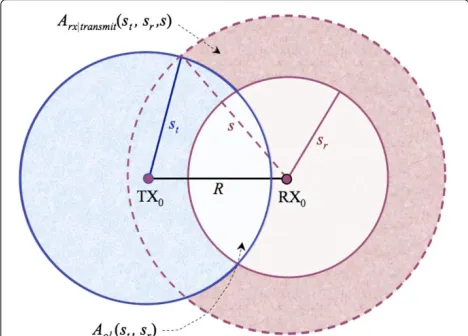
Fol-lowing Equation (4) and the concept of guard zones, we have that if there exists at least one transmission inside B1=B(TX0,st)∪B(RX0,sr)upon the arrival of TX0-RX0,
this transmitter-receiver pair would back off from trans-mission. The area of B1 is shown as the lightly shaded
area in Figure 2, and is given asπs2t +πs2r −Aol(st,sr),
whereAol(st,sr)denotes the area of overlapB(TX0,st)∩
Aol(st,sr)=
Once TX0and RX0jointly decide to transmit, there is
still a probability that their packet is in error upon its arrival due to an ongoing transmission insideB(RX0,s)
that was not detected in the backoff decision-making stage. That is, the packet is in error at the start, if an active transmission is detected inside B(RX0,s) ∩
B(TX0,st)∪B(RX0,sr). This area is marked as the darkly
shaded region in Figure 2, and is given by
Arx|active(st,sr,s)=
Now, given the packet transmission of TX0-RX0is
initi-ated and it is not in error at the start of its transmission, there is a probability that a new interferer, TXi, enters the
plane at somet ∈ (0,T), is located insideB(RX0,s), and
thus causes error for the packet of RX0. Since TXiwould
back off if it or its receiver detect the transmission of TX0,
this means that in order for TXito cause outage for RX0,
it must be placed insideB2=B(RX0,s)∩B(TX0,st), while
its receiver RXiis located outside ofB(TX0,sr). This
prob-ability is denoted asPduring, and is given in the following
subsection.
Due to the Poisson distribution of interferers, we apply the expressionPerror=1−exp{−λcsmaA}, whereAis the
de-Figure 2Geometrical illustration of sensing zonesB(RX0,sr)and B(TX0,st).
tection area depending on the particular error probability to be calculated. Moreover, the densityλcsmais given as
λcsma =
wherePbis the backoff probability,Prt1is the probability
that the packet is received in error at its first transmis-sion attempt, and Prt is the probability that the packet
is received erroneously in a retransmission attempt. The reason we distinguish betweenPrt1andPrtis that due to
the backoff decision making stage, the area where there is a probability of detecting an active interferer during a transmission is smaller in the first transmission than in the following retransmissions.
3.2 Outage probability in non-fading networks
Based on the above derivations, we are now able to math-ematically express the outage probability of CSMATXRX
in a non-fading network. This is given by the following theorem.
Theorem 1.The outage probability of CSMATXRXin the
absence of fading with varying sensing thresholds is given by
Pout(CSMATXRX) = PMb +
1−PMb Prt1PNrt, (9) where:
• Pbis the backoff probability, approximated by the solution to packet is received in error in a retransmission attempt.Prxis the probability that the packet is in error at the start of each of its retransmissions, approximated by
• Pduringis the probability that an error occurs at some
whereGactive(st,sr)is given as the RXiis not in error upon its arrival, are given as
P(active|r,φ)=1−1 probability that the packet is received in error at its first transmission attempt.Prx|activeis the probability that the receiver is in outage at the start of the packet, although it decides to initiate its transmission, approximated by
For more details on the derivation of Equations (10) and (14), please refer to [12]. Optimization of the sens-ing thresholds is carried out in Section 5, and comparison between CSMATXRX with the other CSMA versions is
performed in Section 6.
4 Performance in the presence of fading
In this section, we add fading effects to the path loss attenuation, as described in Section 2. Due to the inde-pendence of the channel fading coefficients on distance, we can no longer operate with the closest interferer for the derivation of the outage probability. Instead, we must consider thedominant interferer, which is a single interferer whose received interference power (affected by the distance and the random channel coefficients) aloneis strong enough to result in outage for the packet under observation.
Similar to Section 3, we first explain the method of analysis as well as the key steps of the mathematical derivations, before the result of the analysis is presented in Subsection 4.2.
4.1 Method of analysis
The outage probability expression in the case of fading is the same as Equation (9), with the difference thatPb,Prt1,
andPrtare replaced by their average values with respect to
the fading coefficients, namelyPb,Prt1, andPrt. Based on
the same reasoning as in the non-fading case in Section 3, the density of packets attempting to access the channel is
λcsma = λ
The probability that a given transmitter-receiver pair, TX0-RX0, backs off is given by the probability that the
SINR at the start of the packet is belowβtat the transmit-ter, or belowβrat the receiver, or both. Hence,
Pb = Pb1(βt)+Pb1(βr)−Pr(TX0beg. ∩ RX0beg.)
(17)
Pb1(βt)andPb1(βr)are derived by using a modified
ver-sion of the guard zone concept discussed in Section 3. With an SINR constraint ofβ ∈ (βt,βr), define the dis-tance to the dominant interferer (given h00 andh0i) as
sf(h00,h0i) = h10/αi
Consequently, we have that the average number of dominant interferers within a distance sf(h00,h0i) away
and with arrival time during(−T, 0)is approximated by π λcsmasf(h00,h0i)2. Due to the Poisson distribution of
packets, the backoff probability then becomes
Assuming a strictly interference-limited network (i.e., η≈0) with Poisson distributed packets, we have
Pb1(β)≈1−exp
that in order to findλactiveonly the first term of Equation
(8) is multiplied by(1−Pb), because once a packet
trans-mission is initiated (the second term in Equation (8)), no further decision-making is performed for each retrans-mission attempt. Furthermore, knowing that for Rayleigh fading channels,E tions, we may apply the result [20]
Eh−002/α
which is inserted back into Equation (20).
To derive the backoff probability, we return to our geometrical analysis again. We assume that B(TX0,sft)
Inserting this expression back into Equation (17), yields the backoff probability of CSMATXRX.
Once a transmission has been initiated, there is a proba-bility that the packet is in error at the start of its first trans-mission attempt. This is denoted by Prx|active(h00,h0i).
Using geometry again, this probability is given as the prob-ability that an active interferer already exist on the plane insideB(RX0,sf), that was not detected during the
back-off decision-making stage. That is, the interferer TXimust
be located insideArx|active(sft,s f
r,sf), which is shown as the
darkly shaded area in Figure 2 and is approximated by Equation (7).
To derive the probability that a packet is received in error at some time during its transmission, denoted by Pduring, we use the Poissonianity of interferers and apply
the following expression:
whereμf is the expected density of dominant interferers, TXi, for the packet at RX0. This is given as
4.2 Outage probability in fading networks
Based on the derivations given above, we arrive at the following theorem.
Theorem 2.The outage probability of CSMATXRXin the
presence of Rayleigh fading with varying sensing thresholds is given by
the average backoff probability, wherePb1(βt)is approximated by the solution to
Pb1(βt)=1−e probability that a packet is received in error in a retransmission attempt.Prxis the average probability that the packet is in error at the start of each of its retransmissions, approximated by • Pduring(h00)is the probability that an error occurs at
somet∈(0,T), approximated by
is the probability that the packet is received in error at its first transmission attempt, withPrx|active(h00)approximated by
Optimization of the sensing thresholds is carried out in the next section, and comparison between CSMATXRX
with the other CSMA versions is performed in Section 6.
5 Optimizing the sensing thresholds
In order to find the optimal sensing thresholds of CSMATXRX,βtopt, andβ
opt
r , such that the outage
proba-bility is minimized, we must in principle differentiate the outage probability expressions given in Theorems 1 and 2 with respect tostandsr, and set each equal to 0. However,
because of the complexity of our equations, this turns out to be a nontrivial task. Hence, we attack our optimization problem from another angle; we evaluate the total out-age probability of CSMATXRXbased on the change in the
exposed and hidden node problems.
The hidden node problemof CSMA occurs during an
active packet transmission when a newly arriving trans-mitter, TXi, is located too close to the receiver under
observation, RX0, while TXiand RXiare simultaneously
too far away from TX0 to detect its transmission. That
is, TXi initiates its transmission and causes outage for
RX0 because TX0 is hidden to it and its receiver. The
probability of such an event occurring is
Pr(hidden node) ≈ Pr(RX0mid.|TXibeg.∩ RXibeg.).
Theexposed node problemoccurs when a packet trans-mission is backed off even though its transtrans-mission would not have contributed to any outages. This is the case when the interferer TXior its receiver RXiare located too close
to the active transmission of TX0, but far enough from
RX0to not cause any errors for it. That is,
Pr(exposed node)≈Pr(TXibeg.∪ RXibeg.| RX0mid.).
The exposed node problem is a direct consequence of the transmitter making the backoff decision.
5.1 Optimization in the absence of fading
In a non-fading network, we note thatPout(CSMATXRX)
is a convex function of st and sr for low densities. As
a simplified proof for this claim, we note that the total outage probability of CSMATXRXmay for high densities
be approximated by the summation of error probability expressions, which are of the formPerror=1−e−λcsmaπs
2
. Differentiating this expression twice with respect to s = {st,sr}yields
d2Perror
ds2 = 2π λcsmae
−π λcsmas2 1−2π λ csmas2
. (31)
For 2π λcsmas2<1, we have that d2Perror
ds2 >0, indicating
convexity. Hence, we may conclude that for low enough values of the density (where our approximate expressions are more accurate),Perror(and therebyPout(CSMATXRX))
is a convex function ofs.
This means that in order to obtainβtoptandβropt
(equiva-lentlysoptt andsoptr ), we may minimize the outage
probabil-ity with respect to each variable separately. Starting from Equation (9), we have that the derivative of the outage probability for arbitrary values ofMandNwith respect to the sensing radiusst(equivalentlysr) is
dPout(CSMATXRX)
dst =
M PM−b 1
1−PN+rt 1
dPb
dst
+(N+1)PrtN(1−PMb )(1−Prx)
×dPduring dst
,
(32)
wherePrt =Prx+(1−Prx)Pduring. The optimal value for
stis then the solution todPout(CSMAdst TXRX) =0, which must
be solved numerically.
In order to find a closed-form expression for the optimal values ofstandsr, we consider the particular case ofM=
1 andN=0. This yields
Pout(CSMATXRX)=
Prx+(1−Prx)Pduring ;sr<s
Pb+(1−Pb)Pduring ; otherwise
(33)
First setstto be a fixed value (e.g.,st=0 as in [12]). We
know from [12] that the optimalsrthat minimizes the
out-age probability of CSMARXissoptr =s, which corresponds
toβropt=β. The intuition behind this is as follows: • Forsr <s⇒B(RX0,sr) <B(RX0,s)⇒lower
probability of backoff⇒higher probability that outage occurs during an active transmission. Note that the reduction in the backoff probability does in fact not result in a reduction in the probability that outage occurs during a transmission, because even thoughB(RX0,sr) <B(RX0,s), any active
transmissions insideB(RX0,s)upon the arrival of TX0-RX0will contribute to the outage. Hence, if
sr<s, the total outage probability will be higher than its minimum value.
• Forsr >s⇒B(RX0,sr) >B(RX0,s)⇒higher probability of backoff⇒lower probability that outage occurs during an active transmission.
circumference of the circle around TXiwhere RXi can be located. Hence, the total outage probability increases assrincreases beyonds.
Assuming thatsoptr = s, we have thatPout(CSMATXRX)
is a function ofstonly. In order to find the optimal sensing
radius of the transmitter,soptt , we use the outage probabil-ity of CSMARXaas a reference. The probability that TX0
is hidden to both TXi and RXi is lower than the
proba-bility that it is hidden only to RXi, which is the case in
CSMARX. Hence, the transmitter sensing of CSMATXRX
reduces the hidden node problem, as the area around RX0
where the activation of an interferer will and cause out-age, is reduced. For a non-fading network, this yields the following approximation:
˜
Pduring ≈ ˜PRXduring − (1−e−λcsmaAol(st,sr)), (34)
whereAol(st,sr)is the area of overlap betweenB(TX0,st)
and B(RX0,sr), as illustrated in Figure 2 and given by
Equation (6). The exposed node problem occurs when TXi-RXi are located inside B(TX0,st), but outside of where P˜RXb is the backoff probability of CSMARX as
derived in [12], andAol(st,sr)is given by Equation (6).
Setting this derivative equal to 0, we obtain:
(1−Pb)e−λAol(st,s thatsoptt = 0, i.e., it is beneficial to have no transmitter
sensing at all, as is the case in CSMARX. Fors > R,soptt
is found numerically as the nonzero solution to Equation (37), which is plotted in Figure 3 forβ = 10 dB. The rea-son we apply a high value forβ (compared to the value of 0 dB that has been applied before), is to emphasize the benefit of the transmitter sensing.
The point where the outage probability is decreas-ing at its highest rate, i.e., the minimum point of
dPout(CSMATXRX)
dst , occurs forst= s−R
b. This corresponds
toβt =
β1/α−1α. For this value ofβt,B(RX0,s)
cov-ers B(TX0,st) completely, meaning that the transmitter
sensing of CSMATXRXintroduces no additional exposed
node problems, while at the same time providing some protection for its receiver, thus reducing the hidden node problem. That is, for s > R, st can be increased up to (s−R)without introducing any exposed node problems, meaning that in CSMATXRXit is always valid thatβtopt ≥
β1/α−1α.
5.2 Optimization in the presence of fading
In the case of fading, the optimization problem becomes more complicated, as we can no longer translate it to a dis-tance problem. Intuitively, we would expect CSMATXRX
to yield an optimal performance whenβr=βandβt=0.
The reason for this is as follows:
• Ifβr > β, the exposed node problem is increased, while the hidden node problem is not reduced (this is partly because we do not consider the aggregate interference power in our derivations). On the other hand, ifβr < β, there is no exposed node problem, but the hidden node problem is higher than when βr=β. Hence,βropt=β.
• Next, we evaluate the benefit that the transmitter sensing of CSMATXRXprovides. Since the channel coefficient from TXito TX0is independent from the channel coefficient from TX0to RXi, the
decision-making of the TXibased on its own channel does not provide much benefit for the packet
reception at its receiver (in terms of the hidden node problem). In fact, the transmitter’s decision to back off from transmission when its receiver wishes to activate it, is only adding to the exposed node problem. Hence,βtopt=0.
First, we find the derivative ofPduring;
Derivative of P
tot
Differentiating the backoff probability, Pb, given by
Theorem 2, yields
r)is given by Equation (6). Note that when (M,N)=(1, 0),Pb1(βt)may be expressed by the Lambert
Inserting these expressions back into Equation (38), the optimal value of βt can be found numerically. This is
shown in Figure 4, where dPout(CSMATXRX)
dβt is plotted as a function of βt for various values ofβr. βtopt is
poten-tially the point where the derivative ofPout(CSMATXRX)
crosses 0. As expected, dPout(CSMATXRX)
dβt is positive for all
βt, meaning that it is always an increasing function ofβt.
In other words, the outage probability of CSMATXRX in
−10 −5 0 5 10 15 20 25 30 0
0.2 0.4 0.6 0.8 1 1.2
TX Sensing Threshold, βt
Derivative of P
tot
dP
tot / dβt for β = 1 and βr = 1
dP
tot / dβt for β = 1 and βr = 0.5
dP
tot / dβt for β = 1 and βr = 2
Figure 4Derivative of the outage probability of CSMATXRXin a fading network as a function ofβt, forβ=0dB.
6 Numerical results
In Figures 5 and 6, the outage probability of CSMATXRX
(and CSMARX for the sake of comparison) are plotted
as a function of the packet arrival densityλ, for a non-fading and a non-fading network, respectively. Firstly, our analytical expressions are validated as they follow the simulation results tightly. Note that in the presence of fading, some discrepancies can be observed between the analytical results and simulations; this is due to the addi-tional source of randomness coming from the channel
coefficients, making the “dominant interferer” approxima-tion used in the derivaapproxima-tions less accurate. However, these deviations occur at high densities corresponding to a high outage probability (>0.3), which is at least an order of magnitude higher than what is often applied in practical networks.
Second, we observe that as the density increases, so does the outage probability, until the network reaches a point of saturation, where Pout ≈ 1. By increasing
the number of backoffs and retransmissions, significant
10−2 10−1 100
10−2
10−1
100
Spatial packet arrival density, λ
Probability of Outage
Simulated CSMA−TXRX Analytical CSMA−TXRX Analytical CSMA−RX M = 1, N = 0
M = 2, N = 1
10−2 10−1 100
10−2
10−1
100
Spatial packet arrival density, λ
Probability of Outage
Simulated CSMA−TXRX Analytical CSMA−TXRX Analytical CSMA−RX M = 1, N = 0
M = 2, N = 1
Figure 6Outage probability of CSMATXRXin a fading network withβt=βr=β=0dB.
performance gain can be obtained. For low densities with (M,N) = (2, 1), the outage probability is up to 10 times lower than when(M,N) = (1, 0). Thirdly, the addition of transmitter sensing in CSMATXRXdoes not appear to
provide any improvement compared to CSMARX. In fact,
CSMARXoutperforms CSMATXRXby up to 20% in
non-fading networks and up to 50% when non-fading is present. This is due to the exposed node problem caused by the transmitter sensing in CSMATXRX. That is, when M is
small, the protection that the transmitter sensing provides does not counterbalance the backoff probability increase it generates.
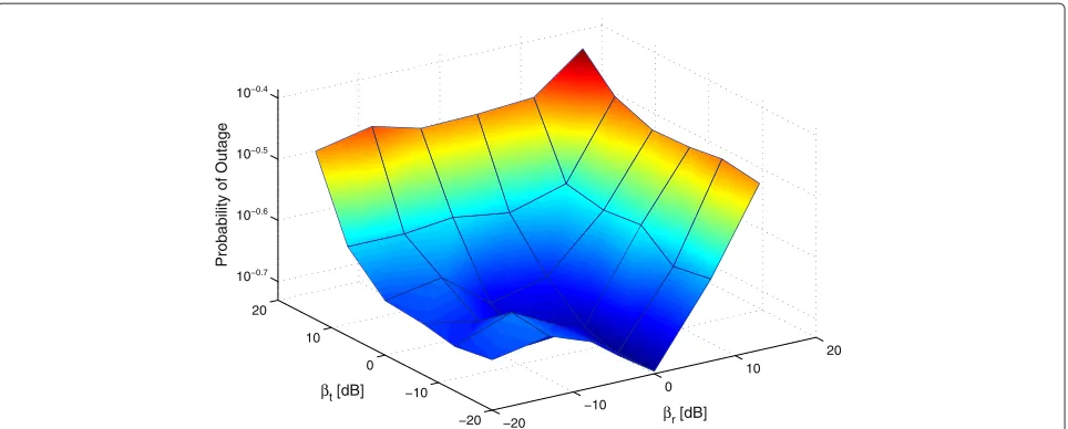
In Figure 7, the outage probability of CSMATXRX
is plotted as a function of the sensing thresholds βt and βr, for a fixed low density of λ=0.01, β =10 dB, and (M,N)=(1, 0). The plot shows that βropt=β =10 andβtopt=5.7 dB, which is also obtained by numerically solving Equation (37), thus confirm-ing our conclusions from Subsection 5.1. Similarly, in Figure 8, the outage probability of CSMATXRX
is considered in a fading network with λ=0.03, β =0 dB, and (M,N)=(1, 0). Again, our derivations from Subsection 5.2 are confirmed, i.e., βropt=β=0 dB
andβtopt=0.
−20 −10
0 10
20 −20
−10 0
10
20 0.1
0.15 0.2 0.25
βt [dB]
βr [dB]
Probability of Outage
βr = 10 dB
βt = 5.8 dB
−20
−10 0
10
20
−20 −10 0 10 20 10−0.7
10−0.6
10−0.5
10−0.4
βr [dB]
βt [dB]
Probability of Outage
Figure 8Outage probability of CSMATXRXas a function of the sensing thresholds, for a fading network withλ=0.03,β=0dB, and (M,N)=(1, 0).
The impact of the number of backoffs, M, is illus-trated in Figure 9, where the receiver sensing threshold is assumed to be constant,βr = β = 0 dB, while Mand the transmitter sensing thresholdβtare optimized jointly. As expected, the outage probability decreases monoton-ically with M. For each M, there is a different value for βtopt, although the range of this is very small. Hence, we conclude that the result of Equation (37) to findsoptt ana-lytically forM = 1, can be applied as an approximation for greater values ofMas well. The fact that outage prob-ability reduces monotonically asMincreases is reinforced in Figure 10, which has the same parameter values as Figure 9.
Figure 11 emphasizes the effect of M on the outage probability of CSMATXRX, as compared to CSMATXand
CSMARX. In this plot, we setN =0 and a high density of
λ = 0.1 is chosen. When onlyM= 1 channel sensing is allowed before the packet is dropped, CSMATXRXexhibits
up to 10% higher outage probability than CSMARX and
up to 20% lower outage probability than CSMATX. As
M increases, the benefit of the joint channel sensing of CSMATXRX becomes more evident; for M = 4,
CSMATXRXoutperforms CSMARXby 40% and CSMATX
by a factor 2. Hence, we conclude that by applying joint transmitter-receiver sensing in a network withM>1, the outage performance of CSMA can be improved beyond
1 2 3 4 −20
−10
0
10
20 10−0.7
10−0.6
10−0.5
10−0.4
10−0.3
Number of backoffs, M TX sensing threshold, βt [dB]
Probability of Outage
Number of Backoffs, M
TX sensing threshold,
βt
1 1.5 2 2.5 3 3.5 4
1 2 3 4 5 6 7 8 9 10
Simulated CSMA−TXRX
Figure 10Contour plot of outage probability of CSMATXRXas a function ofβtandM, for a non-fading network withλ=0.1,
β=βr=0dB, andN=0.
that of CSMARX. Moreover, the optimal sensing
thresh-olds areβropt= βandβtoptis found approximately as the
solution to Equation (37).
The impact of retransmissions is opposite to that of backoffs. As seen from Figure 12, where the outage prob-ability is plotted for a fixed density of λ = 0.03 and M = 2 backoffs, the outage probability of CSMARX
reduces below that of CSMATXRX as the number of
retransmissions,N, increases, e.g., when(M,N) =(2, 0), CSMATXRX outperforms CSMARX by 10%, while for
(M,N) = (2, 3), we have 20% higher outage probability for CSMATXRXthan for CSMARX. While significant gain
is obtained by increasing N from 0 to 2, little benefit is observed forN > 2. Note that we have included results on the impact ofMandNonly in non-fading networks, as similar conclusions are drawn in fading networks.
7 Conclusions
In this article, we improve the performance of CSMA in wireless ad hoc networks by introducing joint
transmitter-1 1.5 2 2.5 3 3.5 4
0.2 0.25 0.3 0.35 0.4 0.45 0.5
Number of backoffs, M
Probability of Outage
Simulated CSMA−TXRX Simulated CSMA−RX Simulated CSMA−TX
0 0.2 0.4 0.6 0.8 1 1.2 1.4 1.6 1.8 2 0
0.02 0.04 0.06 0.08 0.1 0.12
Number of retransmissions, N
Probability of Outage
Simulated CSMA−TXRX Simulated CSMA−RX Simulated CSMA−TX
Figure 12Outage probability of CSMATXRXas a function of the number of retransmissions,N, for a non-fading network withλ=0.03
andM=2.
receiver sensing and simultaneously optimizing the sens-ing thresholds of both the transmitter and the receiver. This protocol is denoted as CSMATXRX. Within a
Pois-son distributed ad hoc network, approximate analyti-cal expressions are derived for the outage probability of CSMATXRXwith respect to the transmission density and
the sensing thresholds. The optimal sensing thresholds for both the transmitter and receiver are obtained both in non-fading and fading networks, and an understand-ing is provided for how these optimal thresholds bal-ance between the hidden and exposed node problems of CSMA. It is shown that using optimal sensing thresholds can provide significant performance gain for all trans-mission densities. Moreover, when multiple backoffs are allowed, CSMATXRX outperforms CSMARX [12], which
was previously shown to provide the best performance in unslotted systems, e.g., whenM = 4, this improvement is 40%.
For future study, we wish to improve the perfor-mance of CSMA by investigating more efficient use and exchange of channel information between each trans-mitter and its receiver. Other possible extensions are to apply adaptive rate and power control to further improve the performance of CSMA in wireless ad hoc networks.
8 Endnotes
aThis protocol was evaluated in [12]. We assume low
density of transmissions, where the outage probability expressions are good approximations.
bThis assumes thats > R, which is the case in most
net-works, as it ensures that the receiver can detect its own transmitter.
Competing interest
The authors declare that they have no competing interests.
Received: 1 August 2011 Accepted: 28 July 2012 Published: 23 August 2012
References
1. L Kleinrock, FA Tobagi, Packet switching in radio channels: Part I - Carrier sense multiple-access modes and their throughput-delay characteristics, IEEE Trans. Commun.23, 1400–1416 (1975)
2. H Ma, R Vijaykumar, S Roy, J Zhu, Optimizing 802.11 wireless mesh networks performance using physical carrier sensing, IEEE/ACM Trans. Network.17(5), 1550–1563 (2009)
3. Y Zhou, SM Nettles, inProc. IEEE Wireless Communications and Networking Conference (WCNC),Balancing the hidden and exposed node problems with power control in csma/ca-based wireless networks, vol 2, (New Orleans, LA, 2005), pp. 683–688
4. G Ferrari, O Tonguz, inProc. IEEE Military Communications Conference,MAC protocols and transport capacity in ad hoc wireless networks: Aloha versus PR-CSMA, vol 2, (Boston, MA, 2003), pp. 1113–1318 5. P Gupta, PR Kumar, The capacity of wireless networks, IEEE Trans. Inf.
Theory.46(2), 388–404 (2000)
6. LL Xie, PR Kumar, On the path-loss attenuation regime for positive cost and linear scaling of transport capacity in wireless networks, IEEE Trans. Inf. Theory.52, 2313–2328 (2006)
7. JA Fuemmeler, NH Vaidya, VV Veeravalli, inUniversity of Illinois at Urbana-Champaign Technical ReportSelecting transmit powers and carrier sense thresholds for CSMA protocols, 2004
8. BJB Fonseca, inProc. Vehicular Technology Conference (VTC),A distributed procedure for carrier sensing threshold adaptation in CSMA-based mobile ad hoc networks, (Dublin, Ireland, 2007), pp. 66–70
10. A Hasan, JG Andrews, The guard zone in wireless ad hoc networks, IEEE Trans. Wirel. Commun.6(3), 897–906 (2005)
11. S Weber, X Yang, J Andrews, G de-Veciana, Transmission capacity of wireless ad hoc networks with outage constraints, IEEE Trans. Inf. Theory. 51(12), 4091–4102 (2005)
12. M Kaynia, N Jindal, GE Øien, Performance analysis and improvement of MAC protocols in wireless ad hoc networks, IEEE Trans. Wirel. Commun. 10, 240–252 (2011)
13. KJ Park, L Kim, JC Hou, inDepartment of Computer Science UIUCDCS-R-2007-2884, University of Illinois at Urbana-Champaign Coordinating the interplay between physical carrier sense and power control in CSMA/CA wireless networks, 2007
14. H Ma, S Roy, inIEEE International Conference on Mobile Ad Hoc and Sensor Systems, MASS,Simple and effective carrier sensing adaptation for multi rate ad-hoc MESH networks, (Vancouver, Canada, 2006), pp. 795–800 15. F Rossetto, M Zorzi, inProc. IEEE Global Communications Conference
(GLOBECOM),Gaussian approximations for carrier sense modeling in wireless ad hoc networks, (Washington, DC, 2007), pp. 864–869 16. K Jeong, H Lim, inProc. AMC CoNEXT,Experimental approach to adaptive
carrier sensing in IEEE 802.15.4 wireless networks, (Madrid, Spain, 2008). article no. 47
17. P Muhlethaler, A Najid, inProc. IEEE European Wireless Conference, Throughput optimization in multihop CSMA mobile ad hoc networks, (Barcelona, Spain, 2004)
18. J Zhu, B Metzler, X Guo, Y Liu, inProc. IEEE INFOCOM,Adaptive CSMA for scalable network capacity in high-density WLAN: a hardware prototyping approach, (Barcelona, Spain, 2006, pp. 1–10
19. M Kaynia, GE Øien, N Jindal, inProc. IEEE International Conference on Wireless Communications and Signal Processing (IC-WCSP),Joint transmitter and receiver carrier sensing capability of CSMA in MANETs, (Nanjing, China, (Best Paper Award), 2009), pp. 1–5
20. S Weber, J Andrews, N Jindal, The effect of fading, channel inversion, and threshold scheduling on ad hoc networks, IEEE Trans. Inf. Theory.53(11), 4127–4149 (2007)
doi:10.1186/1687-1499-2012-271
Cite this article as:Kaynia and Øien:Optimizing the performance of non-fading and non-fading networks using CSMA with joint transmitter and receiver sensing.EURASIP Journal on Wireless Communications and Networking2012
2012:271.
Submit your manuscript to a
journal and benefi t from:
7Convenient online submission
7Rigorous peer review
7Immediate publication on acceptance
7Open access: articles freely available online
7High visibility within the fi eld
7Retaining the copyright to your article