R E S E A R C H
Open Access
End-to-end channel capacity of MAC-PHY
cross-layer multiple-hop MIMO relay system
with outdated CSI
Pham Thanh Hiep
1*, Nguyen Huy Hoang
2, Sugimoto Chika
1and Kohno Ryuji
1Abstract
For high end-to-end channel capacity, the amplify-and-forward scheme multiple-hop multiple-input multiple-output relay system is considered. The distance between each transceiver and the transmit power of each relay are optimized to prevent some relays from being the bottleneck and guarantee high end-to-end channel capacity. According to the proposed transmission environment coefficient, the path loss can be described in a new way, and then the distance of multiple-hop relay system can be optimized more simply than the original one. However, when the system has no control on media access control (MAC) layer, performance of the system deteriorates because of the presence of interference signal. Thus, the specific transmission protocol on the MAC layer for multiple-hop system is proposed to reduce the power of interference signal and to obtain high end-to-end channel capacity. According to the proposed transmission protocol on the MAC layer, the system indicates the trade-off between the end-to-end channel capacity and the delay time. The end-to-end channel capacity of the outdated channel state information system is also analyzed.
1 Introduction
Multiple-input multiple-output (MIMO) relay systems have been discussed in several literatures [1-3]. Addition-ally, ergodic capacity of the amplify-and-forward relay network is discussed. The links between the relay trans-mitters and relay receivers are assumed to be parallel [4] and serial [5,6]. The end-to-end channel capacity based on the different number of antennas at the transmitter, the relay, and the receiver also has been evaluated [5,6]. How-ever, the number of relays considered there (in [5,6]) is only one.
When the number of antennas in relay is less than the number of antennas in the transmitter and receiver, the capacity of MIMO relay system is lower than that of the original MIMO system. Moreover, when the num-ber of antennas in relay equals that in the transmitter and receiver or more, the MIMO relay system can provide the same average capacity as an original MIMO system. In
*Correspondence: [email protected]
1Division of Physics Electrical and Computer Engineering, Graduate School of Engineering, Yokohama National University, Yokohama, Kanagawa Prefecture 240–8501, Japan
Full list of author information is available at the end of the article
other words, although the number of antennas in relay is larger than that in transmitter and receiver, the capacity of MIMO relay system cannot exceed the capacity of original MIMO system [7-10].
Therefore, in order to achieve a high channel capacity, the multiple-hop relay system is considered [11,12]. How-ever, in these papers, the interference signal is assumed to be absent; the performance based on a transmission protocol that only has two phases is analyzed, the signal-to-noise ratio (SNR) at the receiver is assumed to be fixed, and the location as well as the transmit power of each transmitter are not dealt. In the multiple-hop MIMO relay system, when the distance between the source (TX) and the destination (RX) is fixed, the distance between the TX to a relay station (RS), RS to RS, and RS to the RX called the distances between transceivers, is shortened. Conse-quently, according to the number of relay and the location of the relays, the SNR and the capacity are changed. Hence, to achieve the high end-to-end channel capacity, the location of each relay, meaning the distance between each transceiver, needs to be optimized. We have ana-lyzed the performance of half-duplex multiple-hop relay system with the amplify-and-forward strategy [13] and
decode-and-forward strategy [14]. However, the multiple-hop relay system has been optimized on the physical layer, and the transmission of each relay is assumed to be con-trolled accurately. In this paper, the transmission protocol on media access control (MAC) layer is proposed and the multiple-hop relay system is optimized on both physical and MAC layers, the PHY-MAC cross-layer. Additionally, the system is analyzed when the outdated channel state information (CSI) at the receiver is taken into account. The channel capacity in this paper is the ergodic channel capacity.
The rest of the paper is organized as follows. We intro-duce the channel model of perfect CSI multiple-hop MIMO relay system in Section 2. Section 3 is the analy-sis of the system that has interference. The specific access control on the MAC layer is described in Section 4. The end-to-end channel capacity of the outdated system is analyzed in Section 5. Finally, Section 6 concludes the paper.
2 Multiple-hop MIMO relay system 2.1 Channel model
We assume that there are many relay nodes, i.e., mobile phone and personal computer, arranged in a straight line from the base station to the receiver. When the receiver wants to receive the information from the base station, it transmits the request message to the base station via the relay node. After receiving the message from the receiver, the relay node detects the CSI and adds its location information into the message and trans-fers to the other node. When the base station receives the request message, it optimizes the distance and the transmit power based on each transmission protocol of the MAC layer. According to the location information of each relay node added into the message, the base station decides the optimized relay node and its trans-mit power for the multiple-hop relay system. Finally, the base station starts transmitting the information to the receiver.
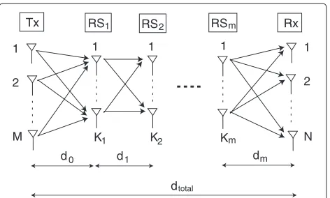
Figure 1 showsmrelays that intervened in the MIMO relay system. Let M, N, and Ki (i = 1,. . ., m) denote the number of the antenna at TX, RX, and RSi, respec-tively. The distance between each transceiver is denoted bydi (i=0,. . ., m). The distance between TX and RX is fixed asdtotal. TX and all of the relays employ the amplify-and-forward strategy. Mathematical notations used in this paper are as follows: xandX are scalar variables;xand Xare vector and matrix variables, respectively;(·)His the conjugate transpose.
For easy description, TX and RX are also denoted as RS0 and RSm+1, respectively. Since path loss is taken into con-sideration, the channel matrix is a composite matrix and is modeled as follows:li,i+1Hi, i = 0,. . ., m, of which
Hirepresents the channel matrix between RSiand RSi+1,
Tx RS Rx
Figure 1The system model of multiple-hop MIMO relay system.
li,j denotes the path loss between RSi and RSj. The path loss is described in detail in the following section.Hiis a matrix with independent and identical distribution (i.i.d), zero mean, unit variance, circularly symmetric complex Gaussian entries.
We assume that the transmit power of TX (ETX) and the total transmit power of relays (ERS) are fixed and are not affected by the change in the number of relays and antennas at each relay. In order to simplify the compo-sition of relay and demonstrate the effect of optimizing the distance and the transmit power of each relay, we assume that the transmit power of each relay is equally divided into each antenna, and the number of antennas in each relay is the same. Moreover, zero-forcing algo-rithm is applied in both the transmitter and the receiver. At first, the system is assumed to be controlled and the interference is absent. All relays transmit the signal at the same time, with full allocation time. Hereafter, this sys-tem is called the ideal syssys-tem, and the end-to-end channel capacity of the ideal system is called the ideal end-to-end channel capacity. After that, the interference between every transceiver is taken into consideration, and the spe-cific access control is proposed to obtain high end-to-end channel capacity.
In the ideal system, the ideal end-to-end channel capac-ity of forward link (from TX to RX) in multiple-hop relay systems is expressed as follows. When the signal si−1 is transmitted from RSi−1, the received signal at RSi is expressed as follows:
si=Hi−iβi−1si−1+ni, (1)
wherepirepresents the transmit power of one antenna of
Whenmrelays are intervened, the signals0is transmitted from TX, and the received signal at RX becomes
sm+1=
where nsystem denotes the noise vector of the system. Therefore, the system channel matrix is written by
H=
pmlm,m+1. . .p0l0,1
|sm|2. . .|s1|2 Hm. . .H1H0. (4)
According to the usage of the system channel matrixH, the multiple-hop MIMO relay system can be analyzed the same as the conventional MIMO system.
2.2 Ideal end-to-end channel capacity
Since amplify-and-forward method is applied to the chan-nel model, the noise is also amplified and transmitted to the next relay. Therefore, the system noise vector whenm relays are intervened becomes as follows:
nsystem=
whereσ2is the covariance of the noise vector in all relays and f(li,i+1,pj,σ2) is a polynomial ofli,i+1,pj,σ2. Since σ2 1 and the covariance of noise vector are smaller than the received power, the component containing σ4
can be ignored. Thus, Equation 6 can be changed to the following:
Consequently, the end-to-end channel capacity of the multiple-hop MIMO relay system is expressed as follows:
C=log2 number of relays, the distance between each transceiver, and the transmit power of each relay. It means that the end-to-end channel capacity is only restricted byfm. Therefore, function fm can be considered instead of the end-to-end channel capacity. In order to achieve the high end-to-end channel capacity, the function fm has to be minimized.
2.3 Path loss
As in Equation 8, the system channel matrix is propor-tional to pi and li,i+1. Therefore, the path loss plays an important role in the channel model. Since there are a lot of obstacles in the propagation environment, such as huge building, it is necessary to consider the path loss as being attenuated by the reflection. The power of signal is reduced, corresponding to the transmission distance and the number of reflections. An amount of the reduc-tion by one-time reflecreduc-tion is called reflecreduc-tion factor. Naturally, the reflection factor is changed according to the shape of obstacles, the angle of reflections, and so on. However, in this paper, the reflection factor of all reflec-tions is assumed to be the same and denoted bya. The path loss is expressed as follows [15-21]:
li,i+1=
coefficient W is defined as the average distance of the line-of-sight distance between each transceiver. There-fore, the reflected number between each transceiver can be expressed asti = Widi and the path loss in Equation 10 can be rewritten in the following new type:
li,i+1=
⎛ ⎝λa
di Wi
4πdi ⎞ ⎠
2
. (11)
According to the new type, the path loss becomes a func-tion of the distance only. Addifunc-tionally, the Taylor
expres-sion is applied into the termaWidi , and then the path loss becomes an equation of higher degree of the distance. Therefore, the distance can be optimized easily by the mathematical method or the particle filter method that be explained in the following section.
3 System that has interference 3.1 System model
Up to now, the interference signal is assumed to be absent and the system has been analyzed. However, when the system has no control on the MAC layer or has incomplete control, the interference signal is present. The received signal at RSi is considered. RSi simulta-neously receives the desired signalsi−1 from RSi−1; the interference signal si−2, from RSi−2; and the interfer-ence signal si+1, from RSi+1. Actually, RSi receives the interference signal not only from the neighbor trans-mitters RSi−2 (forward link) and RSi+1 (backward link), but also from all of the transmitters. However, the inter-ference signal from the other relay is weaker than the interference signal from the neighbor transmitters. Hence, the interference signals from the other relays can be ignored, and the received signal at RSi is expressed as follows:
si=Hi−1isi−1+Hi−2isi−2+Hi+1isi+1+ni, (12)
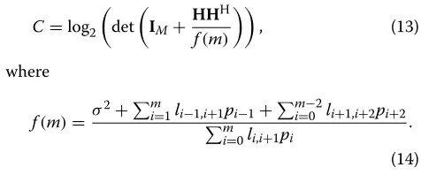
whereHijis the channel matrix between RSjand RSi. Con-sequently, the end-to-end channel capacity of the system has an interference that can be expressed as follows:
C=log2
det
IM+
HHH f(m)
, (13)
where
f(m)= σ
2+m
i=1li−1,i+1pi−1+mi=−02li+1,i+2pi+2
m
i=0li,i+1pi
.
(14)
In comparison with the ideal end-to-end channel capacity, the term of interferencemi=1li−1,ipi−1of the forward link andmi=−02li+1,i+2pi+2of the backward link is added. Sim-ilar to the case of the ideal system, the transmit power and the distance can be optimized by mathematical method [13,14]. However, the optimization distance of the system with difference Wi, especially if the system has interfer-ence, is complicated. In order to easily optimize the dis-tance and the transmit power simultaneously, the particle filter algorithm is applied.
3.2 Particle filter method
In this section, we propose the particle filter (PF) method to optimize both the distance and the transmit powers simultaneously for high end-to-end channel capacity. The algorithm is shown in Figure 2 and explained as follows. LetdandEdenote 1×m+1 distance and transmit power vectors, respectively:
d=[d0, . . ., dm] ,
E=[ETX, E1, . . ., Em] .
(15)
Step 1: 10,000×random samples ofdandEare generated. The functionf for each sample is calculated, and the minimal valuef of all samples is denoted byminf. The sample ofdandEwhich hasminf is called the optimal sample.
Step 2: 10,000×samples ofdandEare generated around the optimal sample by random function.
The functionf for each sample is calculated and is compared tominf.
Step 3: If there is a functionf which is smaller thanminf, thenminf is renewed and the process returns to step 2. Otherwise, the algorithm is finished.
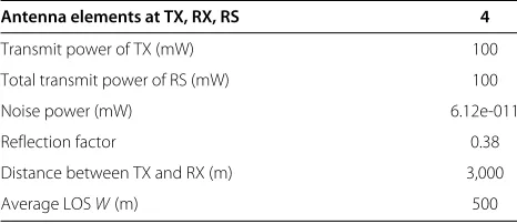
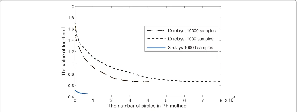
To evaluate the particle filter method, the function f in (14) is calculated with the parameters summarized in Table 1. Figure 3 shows the value of functionf where the number of relays is 3 and 10. In the case where the num-ber of relays is 10, the numnum-ber of samples is changed, i.e., 1,000 and 10,000. As shown in Figure 3, the value of func-tion f decreases when the number of circles increases, and the algorithm is finished when functionf reaches the minimum. The minimum of functionf is achieved in the system with averageW[14]. Therefore, the algorithm can be finished when functionf reaches the value off in the system with averageW.
As shown in Figure 3, we can recognize that the num-ber of circles decreases when the numnum-ber of relays is small and/or the number of samples is larger. However, the PF method requires a large number of samples to converge. If the number of samples is not enough, then the algorithm would not converge or it would take a huge number of circles.
3.3 Numerical evaluation for the system that has interference
The system parameter is summarized in Table 1. In order to evaluate the optimization of distance and trans-mit power. We assume that all relays are arranged in a straight line from the TX to the RX; the transmit power of the RX and the total transmit power of all relays are fixed.
The end-to-end channel capacity of the system in which the transmission of all relays is controlled or not is shown in Figure 4. The end-to-end channel capacity of the system that has interference is much lower than the ideal end-to-end channel capacity. Therefore, in order to obtain the high end-to-end channel capacity, the access control on the MAC layer should be considered
Table 1 Numerical parameters
Antenna elements at TX, RX, RS 4
Transmit power of TX (mW) 100
Total transmit power of RS (mW) 100
Noise power (mW) 6.12e-011
Reflection factor 0.38
Distance between TX and RX (m) 3,000
Average LOSW(m) 500
4 Specific access control on MAC layer 4.1 Multiple-phase transmission
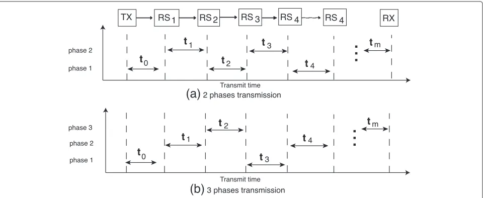
In this paper, the transmission protocol of all relays is assumed to be controlled on time domain. The transmis-sion of all relays is divided into multiple phases of time domain. The relay in the same phase transmits the sig-nal in the same allocation time that is denoted byti. The other relay that will be divided into different phases keeps the silence or receives the signal. Since the neighbor relay transmits the signal in different phases, the interference signal is weaker than that of the system that has no con-trol. Therefore, the end-to-end channel capacity can be respected to be higher.
Figure 5 shows two and three phases of transmis-sion protocol. The two-phase transmistransmis-sion protocol is explained as follows. The even-number relays and the odd-number relays transmit the signal in phases 1 and 2, respectively. Therefore, in the two-phase transmission protocol, the closest interference relays of the backward and forward links to RSiare RSi+1and RSi−3, respectively. The end-to-end channel capacity of the system withn phases can be written as follows:
C=log2
Compare the interference component of the system, it has no control (14) to that of the system withn-phase trans-mission protocol (16), the distance from the interference relay is longer, and the number of interference relay is also larger. Hence, we can say that according to the control on MAC layer, the power of interference decreased; thus, the end-to-end channel capacity is expected to be higher.
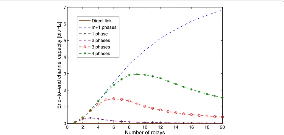
4.2 Numerical evaluation for multiple-phase transmission The allocation time for each phase is assumed to be 1 s, and the system model is the same as the one mentioned. In order to evaluate the transmission protocol on the MAC layer, the distance between each transceiver and the trans-mit power of each relay are assumed to be equal. Figure 6 shows the end-to-end channel capacity in case the access of all relay is controlled on the MAC layer.
signal is taken into account. When the number of relays is small, the distance between each transceiver is large; therefore, the power of interference signal is low and the end-to-end channel capacity is high. Moreover, when the number of relays is large, the power of interference signal increases. Therefore, the signal-to-interference noise ratio (SINR) decreases, and the end-to-end channel capacity decreases.
The end-to-end channel capacity of one-phase and two-phase transmission protocols is almost the same. The rea-son is that, compare to two-phase transmission protocol in Subection 4.1, in one-phase transmission protocol, the closest interference relays of backward link and forward link to RSi are RSi+1 and RSi−2, respectively. Therefore, the power of interference signal to each relay in both phase transmission protocols is almost the same.
The optimum number of relays and the highest end-to-end channel capacity are different for each phase. Since the power of interference signal decreases when the num-ber of phases increases, the end-to-end channel capacity of the higher number of phases is higher than that of lower number of phases. In order to evaluate the multiple-hop relay system, the system without relay node, meaning the direct link from the TX to the RX, is taken into consid-eration. In the case of direct link, the transmit power of TX is 200 mW (the sum of transmit power of TX and all relay nodes); the other parameters are the same as those in the multiple-hop relay system (Table 1). The chan-nel capacity of direct link is 6× 10−4 bit/s/Hz, which is much smaller than that of the multiple-hop relay sys-tem (Figure 6). The reason can be that the signal power is reduced by the distance to the power of 2 and the number of reflections; compared to the direct link, the distance of the multiple-hop relay system is shorter and the number of reflections is smaller. Therefore, although the interfer-ence signal is present, the SINR of the multiple-hop relay
system is higher than the SNR of the direct link. Since the channel capacity of direct link is much smaller than that of the multiple-hop relay system in the proposed propa-gation environment, hereafter, only the channel capacity of the multiple-hop relay system is considered. However, the delay time of each scenario should be considered. The delay time is defined as the delay of transmitted signal to the RX compared to the original MIMO system (the direct link). The delay time of the signal transmitted from the TX to the final receiver RX is described in Figure 7. We can recognize that the delay time increases when the num-ber of relays as well as the numnum-ber of phases increase. It is the trade-off between the end-to-end channel capacity and the delay time.
As shown in Figures 4 and 6, the end-to-end chan-nel capacity of the system that has control on the MAC layer is higher than that of the system that has no con-trol. However, it is smaller than the ideal end-to-end channel capacity. In order to obtain the higher end-to-end channel capacity, the distance and the transmit power should be optimized based on each transmission protocol on the MAC layer or the MAC-PHY cross-layer.
4.3 Numerical evaluation for MAC-PHY cross-layer For MAC-PHY cross-layer, for each transmission pro-tocol on the MAC layer, the distance and the trans-mit power are optimized simultaneously by particle filter method (Subsection 3.2). The allocation time for each phase is assumed to be 1 s, and the system model is the same as mentioned. The end-to-end chan-nel capacity of the MAC-PHY cross-layer is shown in Figure 8.
Similar to the system that only has control on the MAC layer, there is the optimum number of relays which achieves the highest end-to-end channel capacity and the
0 1 2 3 4 5 6 7 8 x 10⁴
0.4 0.6 0.8 1
1.2
1.4 1.6
1.8
2
The number of circles in PF method
The value of function f
10 relays, 1000 samples
3 relays 10000 samples 10 relays, 10000 samples
5 10 15 20 25 30 0
2 4 6 8 10 12
Number of relay nodes
End-to-end
channel
capacity
[bit/Hz]
Without interference With interference
Figure 4Comparing the end-to-end channel capacity of the ideal system and the system that has interference.
trade-off of channel capacity-delay time. However, com-paring to the system that has equal distance and transmit power (Figure 6), the end-to-end channel capacity of the system with MAC-PHY cross-layer is much higher.
Up to now, since the transmission of relay node is assumed to be isotropic, there is the interference from both forward link and backward link. However, the MIMO relay node can use the beamforming technique to transmit the signal to the next relay. It means that the sig-nal is transmitted to the forward link only and that the interference from the backward link is absent. Figure 9 shows the end-to-end channel capacity of system that only has the forward link interference.
As shown in Figure 9, the end-to-end channel capacity increases when the transmission phase increases. Addi-tionally, the trade-off of the channel capacity-delay time
can be applied to this scenario. However, comparing to the system that has interference from both forward link and backward link (Figure 8), the end-to-end channel capacity of the system that only has the forward link interfer-ence (Figure 9) is much higher. It means that there is the trade-off between complication and channel capacity. The beamforming of MIMO can be applied in the scenario that the higher channel capacity is requested and that the device is large enough to equip the MIMO beamforming.
Up to now, the allocation time of each phase is assumed to be 1 s. Thus, there is the trade-off between the channel capacity and the delay time. However, when the trans-mission time is normalized, it means that the time to transmit the signal from the TX to the final receiver RX is fixed at 1 s and the allocation time of each phase is changed, depending on the number of phases. The
RS1 RS2 RX
TX
t
0
t t
1 m
(a)
2 phases transmission phase 1phase 2
RS3 RS
4 RS4
t
t
3
2 t4
t
0
t
t
1
m
phase 1 phase 2 phase 3
t t
3 2
t4
(b)
3 phases transmission Transmit time Transmit time0 2 4 6 8 10 12 14 16 18 20 0
1 2 3 4 5 6 7
Number of relays
End−to−end channel capacity [bit/Hz]
Direct link m+1 phases 1 phase 2 phases 3 phases 4 phases
Figure 6End-to-end channel capacity of the system that has access control on MAC layer.It is compared to the channel capacity of the direct link.
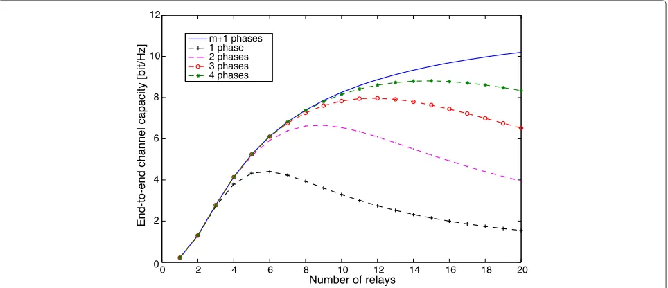
larger the number of phases, the smaller the allocation time of each phase becomes. The system model is the same as mentioned, and the relationship between the end-to-end channel capacity and the number of relays when the transmission time is normalized, as shown in Figure 10. In this system, we also assume that MIMO beamforming is applied for all relays; therefore, only the interference from the forward link is taken into account.
As shown in Figure 10, there are the optimal numbers of relays in the sense of maximal end-to-end channel capac-ity of each number of phases. Additionally, the maximal end-to-end channel capacity and the optimal number of relays are changed, depending on the transmit power of TX, the total transmit power of RS, the transmission envi-ronment (W), and so on. In the case where the number of relays is small, the optimization of the system has no con-trol on the MAC layer (all relays transmit the signal at the
0 2 4 6 8 10 12 14 16 18 20
0 5 10 15 20 25 30 35 40 45
Number of relays
Delay time [s]
1 phase 2 phases
3 phases 4 phases m+1 phases
Direct link
0 2 4 6 8 10 12 14 16 18 20 0
2 4 6 8 10 12
Number of relays
End-to-end channel capacity [bit/Hz]
m+1 phases 1 phase 2 phases 3 phases 4 phases
Figure 8The end-to-end channel capacity of MAC-PHY cross-layer.
same time, one phase) which can reach the higher end-to-end channel capacity than in other scenarios. Moreover, in the case where the number of relays is large, the higher number of phases can obtain the higher end-to-end chan-nel capacity. Hence, to obtain the high end-to-end chanchan-nel capacity, the appropriate number of relays, the number of phases, and so on should be adopted.
5 Outdated CSI system 5.1 System model
Up to now, the performance of the system is analyzed under the assumption of a perfect CSI at both the trans-mitter and receiver. However, in actuality, the perfect CSI
assumption is not always practical due to channel esti-mation errors, feedback channel delay, and noise. Com-pared to channel estimation errors, the CSI imperfection introduced by feedback channel delay is sometimes more significant and inevitable.
To characterize the outdated CSI at the RSi, the chan-nel time variation is described by the first-order Markov process:
Hi(t)=ρHi(t−τ )+kH¯i(t), (18)
whereτ denotes the total delay caused by signal process-ing, feedback, and other system delays,ρ = J0(2πfDτ ) is the time correlation coefficient,J0(·) is the zero-order
0 2 4 6 8 10 12 14 16 18 20
0 2 4 6 8 10 12
Number of relays
End-to-end channel capacity [bit/Hz]
m+1 phases 1 phase 2 phases 3 phases 4 phases
0 2 4 6 8 10 12 14 16 18 20 0
0.1 0.2 0.3 0.4 0.5 0.6 0.7 0.8
Number of relays
End-to-end channel capacity [bit/s/Hz]
m+1 phases 1 phase 2 phases 3 phases 4 phases
Figure 10End-to-end channel capacity of the system that has optimization on MAC-PHY cross-layer when transmission time is normalized.
Bessel function of the first kind andfDdenotes the max-imum Doppler frequency shift. k denotes1−ρ2. The innovation termH¯ialso has i.i.d entries, zero mean, and unit variance. For notation brevity, we drop off the time index:
Hi=ρHˆi+kH¯i, (19)
whereHˆidenotes the outdated channel matrix whileHiis the true one.
We assume that the transmitter adds the CSI in the data packet and transmits to the receiver; thus, the receiver knows both Hi andHˆi. After receiving the data packet, the receiver feedbacks the CSI to the transmitter immedi-ately. However, the transmitter should wait some phases to transmit the signal; therefore, this CSI becomes the out-dated CSI. It means that the transmitter only knows the outdated CSIHˆi, while the receiver knows bothHiandHˆi. In an SVD-based MIMO system, the relay RSi steers the modulated signal vectorsiwithin the eigenspace spanned by the right singular vectors contained inEˆti:
sti = ˆEtisi. (20)
The relay RSi+1receives the signal the same way as that in Subsection 2.1:
sri+1=Hiβisti+ni+1, (21)
and it preprocessessri+1usingEˆri+1:
si+1=(Eˆri+1)Hsri+1,
=(Eˆri+1)HHiβiEˆitsi+(Eˆri+1)Hni+1,
=ρDˆi+1βisi+k(Eˆri+1)HH¯iβiEˆtisi+(Eˆri+1)Hni+1. (22)
We can also use mode complex algorithms such as min-imum mean squared errors or maxmin-imum likelihood to achieve better performance at the cost of higher complex-ity. A basic conclusion is that the more complex methods do perform better in outdated CSI condition. However, the improvement is limited and is at the cost of higher complexity. We use this method for its low complexity and ease of analysis. Thelth component of vectorxand the lth row of matrix x are denoted by x(l) and X(l), respectively. The component-wise form is expressed as follows:
si+1(l)=βi
ρDˆi+1(l)+k(Eˆir+1)HH¯iEˆti(l)
si
+kβi
t=l
(Eˆri+1)HH¯iEˆti(t)si+(Eˆri+1)Hni+1(l),
(23)
where the received signal consists of three components: the information-carrying term, the interference term, and the noise term. The correlation matrix is approximate to the unit matrix. Therefore, the end-to-end channel capacity of n phase outdated CSI system is changed as follows:
C=Mlog2
1+ 1 f(m)
, (24)
0.05 0.1 0.15 0.2 0.25 0.3 0.35 0.4 1
1.5 2 2.5 3 3.5 4 4.5
End−to−end channel capacity [bit/Hz]
m+1 phases 1 phase 2 phases 3 phases 4 phases
Figure 11The end-to-end channel capacity of outdated CSI system that only has forward link interference.There were four relays.
f(m)≈ σ
2+k(M−1)m
i=0li,i+1pi+im=+11−nli−1,i+npi−1+mi=−01−nli,i+1+npi+1+n m
i=0li,i+1pi
, (25)
for the system that has interference from both forward link and backward link.
f(m)≈σ
2+k(M−1)m
i=0li,i+1pi+im=+11−nli−1,i+npi−1
m i=0li,i+1pi
,
(26)
for the system that has interference from only forward link (using MIMO beamforming).
Compared to the system that has perfect CSI at both the transmitter and the receiver (14), in the end-to-end chan-nel capacity of the system that has outdated CSI at the transmitter (26), the co-channel interference by outdated CSI is added.
0.05 0.1 0.15 0.2 0.25 0.3 0.35 0.4
0.1 0.2 0.3 0.4 0.5 0.6 0.7 0.8
End−to−end channel capacity [bit/s/Hz]
1 phase 2 phases 3 phases 4 phases m+1 phases
0 0.05 0.1 0.15 0.2 0.25 0.3 0.35 0.4 1
2 3 4 5 6 7 8
End−to−end channel capacity [bit/Hz]
m+1 phases 1 phase 2 phases 3 phases 4 phases
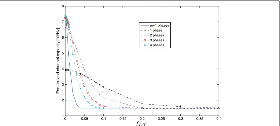
Figure 13The end-to-end channel capacity of outdated CSI system that only has forward link interference.The were eight relays.
5.2 End-to-end channel capacity of outdated CSI system The distance and the transmit power of the outdated CSI system is optimized by particle method (Subsection 3.2). The system model is the same as the one mentioned. The parameter is summarized in Table 1. As explained, the end-to-end channel capacity is changed depending on the number of relays. However, in this section, the end-to-end channel capacity, depend-to-ending on the outdated CSI, is examined. Therefore, we fix the number of relays.
Figures 11 and 12 show the end-to-end channel capac-ity of the system that only has the interference from the forward link (using the MIMO beam forming) where there are four numbers of relays. The end-to-end channel capacity of the system in the case where the transmission time is normalized is shown in Figure 12.
As shown in Figures 11 and 12, the end-to-end chan-nel capacity is decreased when the termfDτ increases. It can be explained that when the term fDτ increases, the power of interference signal is increased; therefore, SINR decreases. The decrease of end-to-end channel capacity in each number of phases is different regardless of how large the end-to-end channel capacity is in the case of the perfect CSI system. The higher the number of phases, the larger the delay time becomes. Therefore, the end-to-end channel capacity of the system has the higher number of phases that decreased more rapidly. It means that the one-phase transmission protocol is the most robust regardless of the number of relays. Figure 13 shows the end-to-end channel capacity of eight relay systems. Although the end-to-end channel capacity of the one-phase system in the case of the perfect CSI (or when the termfDτ is small) is lower than that of the higher number of phase systems,
it becomes higher than the other higher number of phase systems when the termfDτincreases.
6 Conclusions
In this paper, we analyzed the end-to-end channel capac-ity of multiple-hop MIMO relay system with MAC-PHY cross-layer. Compared to the system that has no control on the MAC layer, the end-to-end channel capacity of the system that has control on the MAC-PHY cross-layer is higher. It means that the trade-off of channel capacity-complication is indicated. There is the optimum number of relays for each access control on the MAC layer that achieves the maximal end-to-end channel capacity. How-ever, there is the trade-off between channel capacity and delay time. The system with outdated CSI is also analyzed, and the end-to-end channel capacity of the low number of phases is more robust than that of the higher number of phases regardless of the number of relays.
However, in this paper, the ergodic channel capacity has been analyzed, and we only proposed the MAC layer pro-tocol; the appropriate modulation and code word were not considered. In the future, real-time channel capacity, the appropriate modulation, and code word will be examined. In addition, the optimal combination of the MAC layer and physical layer will be analyzed.
Competing interests
The authors declare that they have no competing interests.
Author details
1Division of Physics Electrical and Computer Engineering, Graduate School of
Received: 17 December 2012 Accepted: 15 May 2013 Published: 29 May 2013
References
1. B Wang, J Zhang, A host-Madsen, On the capacity of MIMO relay channel. IEEE Trans. Inf. Theory.51(1), 29–43 (2005)
2. DS Shiu, GJ Foschini, MJ Gans, JM Kahn, Fading correlation and its effect on the capacity of multi-element antenna systems. IEEE Trans. Commun.
48(3), 502–513 (2000)
3. D Gesbert, H Bolcskei, DA Gore, AJ Paulraj, MIMO wireless channel: capacity and performance prediction. Proc. GLOBECOM.2, 1083–1088 (2000)
4. Y Liang, V Veeravalli, Gaussian Orthogonal relay channels: optimal resource allocation and capacity. IEEE Trans Inf. Theory.51(9), 3284–3289 (2005)
5. K Lee, J Kim, G Caire, I Lee, Asymptotic ergodic capacity analysis for MIMO amplify-and-forward relay networks. IEEE Trans. Commun.9, 2712–2717 (2010)
6. S Jin, M McKay, C Zhong, K Wong, Ergodic capacity analysis of amplify-and-forward MIMO dual-hop systems. IEEE Trans. Inf. Theory.
56(5), 2204–2224 (2010)
7. M Gastpar, M Vetterli, On the capacity of large Gaussian relay networks. IEEE Trans. Inf. Theory.51(3), 765–779 (2005)
8. M Tsuruta, Y Karasawa, Multi-keyhole model for MIMO repeater system evaluation. IEICE Trans. Commun.J89-B(9), 1746–1754 (2006)
9. D Chizhik, GJ Foschini, MJ Gans, RA Valenzuela, Keyholes, correlations, and capacities of multi-element transmit and receive antennas. IEEE Trans. Wireless Commun.1(2), 361–368 (2002)
10. G Levin, S Loyka, On the outage capacity distribution of correlated keyhole MIMO channels. IEEE Trans. Inf. Theory.54(7), 3232–3245 (2010) 11. D Giindiiz, M Khojastepour, A Goldsmith, H Poor, Multi-hop MIMO relay
networks: diversity-multiplexing trade off analysis. IEEE Trans. Wireless Commun.9(5), 1738–1747 (2010)
12. P Razaghi, W Yu, Parity forwarding for multiple-relay networks. IEEE Trans. Inf. Theory.55(1), 158–173 (2009)
13. P Hiep, R Kohno, Optimizing position of repeaters in distributed MIMO repeater system for large capacity. IEICE Trans. Commun.E93-B(12), 3616–3623 (2010)
14. PT Hiep, O Fumie, K Ryuji, Optimizing distance, transmit power and allocation time for reliable multi-hop relay system. EURASIP Journal on Wireless Communications and Networking.2012, 153 (2012) 15. ITU-R, inRecommendation ITU-R P.526-8: propagation by diffraction.
Radiowave Propagation (ITU-R Geneva, 2003)
16. ITU-R, inRecommendation ITU-R P.676-9: attenuation by atmospheric gases. Radiowave Propagation
(ITU-R Geneva, 2001)
17. ITU-R, inRecommendation ITU-R P.838-2: Specific attenuation model for rain
for use in prediction methods. Radiowave Propagation (ITU-R Geneva, 2001)
18. ITU-R, inRecommendation ITU-R P.1057-1: probability distributions relevant
to radiowave propagation modelling. Radiowave Propagation (ITU-R
Geneva, 2001)
19. ITU-R, inRecommendation ITU-R P.1238-3: propagation data and prediction methods for the planning of indoor radiocommunication systems and radio
local area networks in the frequency range 900 MHz to 100 GHz. Radiowave
Propagation (ITU-R Geneva, 2003)
20. ITU-R, inRecommendation ITU-R P.1411-2: propagation data and prediction methods for the planning of short-range outdoor radiocommunication systems and radio local area networks in the frequency range 300 MHz to 100 GHz. Radiowave Propagation (ITU-R Geneva, 2003)
21. N Kita, W Yamada, S Akio, Path loss prediction model for the over-rooftop propagation environment of microwave band in suburban areas. (in Japanese) IEICE Trans.Commun, J89-B(2), 115–125 (2006)
doi:10.1186/1687-1499-2013-144
Cite this article as:Thanh Hiep et al.:End-to-end channel capacity of MAC-PHY cross-layer multiple-hop MIMO relay system with outdated CSI.
EURASIP Journal on Wireless Communications and Networking20132013:144.
Submit your manuscript to a
journal and benefi t from:
7Convenient online submission 7Rigorous peer review
7Immediate publication on acceptance 7Open access: articles freely available online 7High visibility within the fi eld
7Retaining the copyright to your article