R E S E A R C H
Open Access
Node selection algorithm based on Fisher
information
Fei Zhou
1,2and Guan Wang
1*Abstract
Traditional positioning needs lots of measurements between the target and anchors. However, this requirement is faced with significant challenge in the most practical scenarios. The cooperation between mobile nodes is an
effective solution. In order to avoid large computational complexity, we need to cooperate with neighbors selectively. This paper proposes a novel node selection algorithm based on the Fisher information matrix. We represented cooperation information with the equivalent Fisher information matrix and then selected neighbors. Simulation results show that the proposed algorithm is able to improve positioning accuracy obviously compared with distance-based node selection algorithm.
Keywords: Cooperative positioning, Fisher information, Information quantization, Node selection
1 Introduction
Wireless positioning technology is necessary for a large number of new and traditional applications. In a wire-less sensor network, we usually distinguish two different types of nodes: anchor with known position and mobile node with unknown position. Traditionally, mobile nodes need to get at least three measurements from the anchor for positioning. Two traditional positioning methods are the global positioning system (GPS) [1] and beacon posi-tioning [2]. However, GPS is not effective in some harsh environment, such as indoor or underground, because of the obstacles. Beacon positioning is based on the anchor located on the land, for example, WiFi access point and base station. However, these conditions cannot be satis-fied in some cases. Considering the cost, increasing the number of anchor is unrealistic in these complex environ-ments. In addition, since mobile node is battery powered, taking into account energy saving [3–6], communica-tion radius of nodes cannot be increased unlimitedly. Cooperative positioning can overcome the traditional restriction. But information exchange and fusion would inevitably bring about large computational complexity
*Correspondence: [email protected]
1Chongqing Key Laboratory of Optical Communication and Networks, Chongqing University of Posts and Telecommunications, Chongwen Road, 400065 Chongqing, China
Full list of author information is available at the end of the article
and communication burden. In fact, some measurements from the neighbors cannot improve the positioning accu-racy but increase the computational complexity. That means that some cooperation information are redundant. So it is necessary to select neighbors which are beneficial to the target. Some common cooperative positioning algo-rithms also considered the node selection [7]. But those node selection algorithms are based on distance. Position-ing accuracy of node selection based on distance is low. Based on the theory of Fisher information matrix (FIM), this paper uses FIM for node selection.
The remainder of this paper is organized as follows. Section 2 introduces the system model. Section 3 presents the information decomposition. Section 4 describes the proposed algorithm. Section 5 presents the simulation results. The conclusion and future work are discussed in the last section.
2 System model
2.1 Signal model
We assume that a network is consists ofNamobile nodes andNbanchors, denoted byNa = {1, 2. . .Na}andNb= {1, 2. . .Nb}, respectively. Common signal model is mea-surement based on receiving signal, for example, angle and distance. The measurement of distance from thekth
node (k∈Na) to the jth node sents the location of node in a 2-D plain. Different from Eq. 1, we select the original signal as measurement. The signal model is written as
zkj(t)= and amplitude of the lth path, respectively, Lkj is the number of multipath components, andvkj(t)is the obser-vation noise. We introduceX as the vector of unknown parameters.
Besides, we introduceZas the observation vector
Z= is obtained from the Karhunen−Loeve (KL) expansion of zkj(t)[8].
. The mean square error satisfies the information inequality [9].
where X consists of two parts: location and channel parameters. Considering the independence of location information and channel parameters, so we ignore chan-nel parameters and simplify the expression of JX. The simplified FIM is a 2Na ×2Na diagonal matrix if in a
2-D environment we called it the equivalent Fisher infor-mation matrix (EFI)[10]. Combing with Eq. 5, the mean square error can be written as follows:
EZ,X
Definition 1 (SPEB [11])The squared position error bound of the kthmobile node in the network is defined to be
3 Information decomposition and quantization 3.1 Decomposition of FIM
In order to analyze the relationship between position-ing accuracy and cooperation information. We need to break down the positioning information of the entire net-work. Bayesian methods deal with estimation problem by establishing the posterior probability density function of the current state with measurements. Once the posterior probability density function is obtained, a minimum mean square error estimation and maximum posterior proba-bility density estimation can be accomplished by compute mean and mode, respectively.
Assuming that the observation sequence z and esti-mation sequencexare Markov sequences. Based on the Bayesian rule, update the posterior probability density of each node can be performed in two steps:
1. Prediction:
Using the fact that the measurements of different nodes are independent and the Markov assumptions are
where z(rel1:T) is inter-node measurements and z(self1:T) is intra-node measurements. Substituting Eqs. 11 and 12 into Eq. 10, it is rewritten as follows:
px(0:T)|z(1:T) cooperation information, spatial cooperation informa-tion, and prior knowledge, respectively. This article do not consider temporal cooperation, so we just break downTt=1p
z(relt)|x(t)
. Because spatial information only associate with a time step, we need not to consider the sequence. Since the measurements of different nodes are independent, then the spatial information ofkth(k∈Na) node is broke down
pzkj|x
Then, the FIM of spatial cooperation information can be decomposed into the following three parts [12]:
JX =JXP+JXA+JXC, (15)
where JXP, JXA, and JXC correspond to a prior knowl-edge, neighboring anchor, and neighboring mobile node, respectively.
3.2 Decomposition and presentation of EFI
We will further decompose the EFI. Similarly, ranging information intensity (RII)λkj [13]and ranging direction matrix (RDM)Jr
φkj
[13] between nodeskandjare intro-duced to express the EFI. Assuming that a priori knowl-edge of node is unavailable, the EFI can be decomposed into two basic building blocks:
JeApk=
and Cjk are associated with anchor and mobile node, respectively.
Through the above analysis, we make the following conclusions:
• Large amount of node information means a small positioning error.
• Each node newly introduced can increase the information, meanwhile reduce the positioning error. • Cooperation information can be represented by RII
and RDM.
• There are many factors affecting the localization error including the distribution of nodes and the channel quality.
4 Node selection algorithm
Cooperation localization algorithm makes nodes share information with each other; the key of the algorithm is to quantify the uncertainty of the cooperation information.
4.1 Node selection algorithm based on distance
Because cooperative information may come from anchor or mobile node. We want to consider not only the error of measurements between nodes but also the error caused by inaccuracy of neighboring mobile node. If there are no appropriate methods to quantify uncertainty of mobile node, positioning error is likely to be magnified. Litera-ture [14] quantified the uncertainty employing position estimated covariance matrix:
where σm2,n corresponds to the intrinsic range measure-ment variance between node mandnand tr(σn2) is the trace of the position estimated covariance matrix. If node n is an anchor, tr(σn2) = 0. Consequently, great tr(σn2) means that nodenhas a small effect on nodem. Thus, this method will minimize the impact of the node with large error, while maximizing the effect of nodes with small error.
There was another method to quantify uncertainty for cooperative tracking of nodes. Supposing node i is the target, node j is a neighbor ofi. If node jis an anchor, then its true locationpj(k)can be used. Otherwise, only a predicted positionpj(k|k−1)is known, which will bring out great positioning error. In order to quantify the error, the literature [15] redefined a new measurement model. Equation (1) was expanded around the predicted loca-tionpj(k|k−1)of nodejusing a first-order Taylor series the first-order partial of derivative ofrij(k)evaluated at
pj(k|k − 1). The proposed algorithm is based on EFI, containing comprehensive factors that affect positioning accuracy. Because EFI and SPEB have a direct relation-ship, we can select neighbors that are advantageous to the target according to EFI.
4.2 Cooperation based on EFI
communicates with neighboring anchors, the EFI can be written as [16] follows:
Je
whereμis the bigger eigenvalue indicating the principal information,ηis the smaller eigenvalue indicating the sec-ondary information, and vis a rotation angle indicating the direction of the principal information. Since the EFI can be diagonalized into a diagonal matrix, combing with Eq. (8), the SPEB is
P(p)= 1
μ+
1
η. (21)
Next, we would analyze how neighboring anchor affects the positioning error.F(μ,η,v)andF(a, 0,φ)are the EFI of the target and a neighboring anchor, respectively. Obvi-ously, information from a anchor is 1-D, along the direc-tionφ. When target receives the information from anchor, EFI will be updatedFμ˜,η˜,v˜=F(μ,η,v)+F(a, 0,φ).
Substituting Eq. 23 into Eq. 22, the two eigenvectors and rotation angle can be calculated.
˜
v=arctanB
A+v. (24)
We can compute the updated SPEB by Eq. 21 and con-clude that SPEB has a relationship with RII and RDM. When the target cooperates with a neighboring mobile node, it would be more complicated. We supposed that JeAp1 = F(μ1,η1,v1),JeAp2 = F(μ2,η2,v2)are the and RDM between node 1 and node 2.
Fμ˜,η˜,v˜=F(μ1,η1,v1)+F We can see that 0< ξ1,2≤1, it represents the uncertainty
resulting from neighboring mobile node. Similarly, we can obtain theμ˜,η˜, and˜vaccording to Eqs. 23 and 24, then calculate the SPEB.
4.3 Neighbor selection algorithm based on EFI
We assume that the target trajectory is fixed. There are a large number of neighbors around target, containing mobile node and anchor. In view of power consump-tion, we select neighbors within a communication range denoted by Rk. In addition, the number of cooperative nodes also has been set to beNmin. These two parameters are dependent on the circumstance and density of the net-work node. Besides, the value will be different according to the requirement of the positioning accuracy. In general, Nminis at least equal to 3.Zk = {zk,1. . .zk,k−1zk,k+1. . .} is the neighbor set of k node and its size is not fixed.
Zkcontains all the information about the neighbors. The neighbor selection algorithm took as inputs:Zk, that was used to calculate EFI for each node and then obtained SPEB. As outputs, setNk of the selected neighbors were obtained. The whole algorithm is reported as a pseudo code in Algorithm 1.
In Algorithm 1, if the cardinality N of the set Zk is greater than or equal to Nmin, the algorithm selects the neighbor subset with smaller SPEB. Note that R0 is set as the smallest communication range. On the contrary, if N is less than Nmin, there are not enough measure-ments to locate the mobile node and the communica-tion range is simply increased by R, whose value is chosen according to the node density of the network. As reported in row 7 of Algorithm 1, we must dis-tinguish between neighboring anchors and neighboring mobile nodes. If neighbor is not a anchor, ξk,i must be computed.
Algorithm 1Neighbors selection algorithm
1: Input:Zk
2: Output:Nk
3: |Zk| = N represents the cardinality of set Zk, set Nmin=5,Rk =R0
4: Calculate the number of neighbors 5: ifN≥ Nminthen ascending order according toSPEBi
10: The output is:Nk =Zk(1 :Nmin)
11: end for
12: elseSetRk =R0+R
2 4 6 8 10 12 14 0
2 4 6 8 10 12
x/m
y/m
Moblie anchor Target Fixed anchor Fixed unknown node
Fig. 1Network deployment of a target and three different neighbors
5 Simulation results
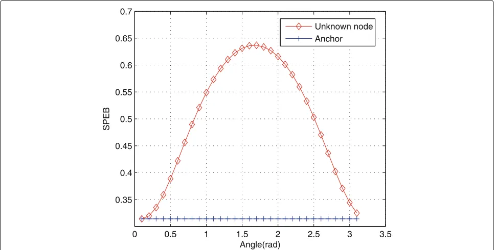
Our simulation results have been carried out in a 2-D environment of size 100 × 100 m. Firstly, there are a target numbered 1, a fixed unknown node numbered 2, a mobile anchor numbered 3 moving around node 2 along a circumference, and a fixed anchor numbered 4 (Fig. 1). Nodes 2 and 4 are neighbors of node 1,
and node 3 is a neighbor of node 2. Seen from Fig. 2, when the angle is equal to 0 and π, nodes 1, 2, and 3 are collinear and v2 = φ1,2. When v2 = φ1,2, ξ1,2 = 1. In this case, error from node 2 is minimal and the SPEB of node 1 is minimal. Besides, the horizontal line indicates that the SPEB in case node 2 is also an anchor.
0 0.5 1 1.5 2 2.5 3 3.5
0.35 0.4 0.45 0.5 0.55 0.6 0.65 0.7
Angle(rad)
SPEB
Unknown node Anchor
0 20 40 60 80 100 0
10 20 30 40 50 60 70 80 90 100
x/m
y/m
Target Anchor:0−50 Anchor:0−25 Anchor:25−50
Fig. 3Neighbor distribution depending on the distance to target
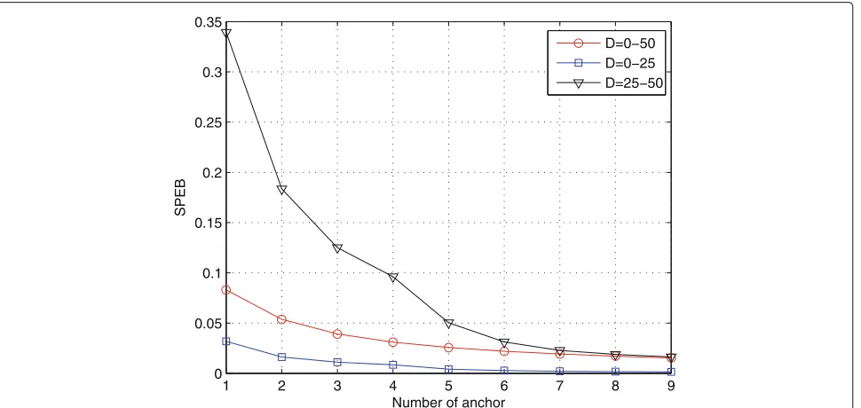
Secondly, all neighboring nodes are distributed on a straight line. According to the distance to the target, neighbors have been divided into three types: 0 − 25, 25−50, and 0−50 (Fig. 3). Since all nodes are located in the same straight line, the effect of the angle on SPEB can be ignored. Seen from Fig. 4, the SPEB is inversely pro-portional to distance and propro-portional to the number of neighbors.
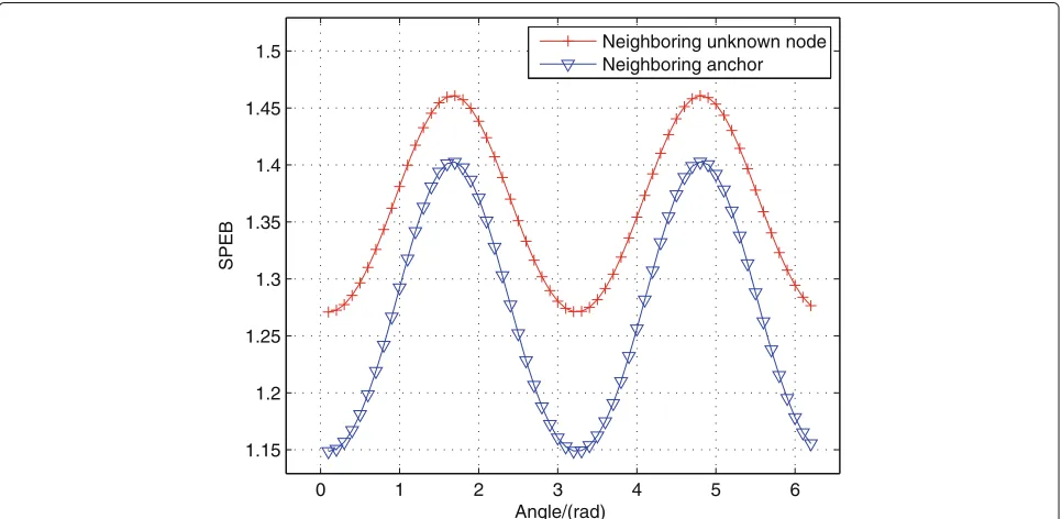
Assuming that a target and a neighboring anchor are fixed. In addition, there are two nodes moving around the target. They do circular motion around the tar-get with radius of 4 and 5, respectively (Fig. 5). And the target only can communicate with the nearer one, but the two moving nodes can communicate. Initial EFI of the target is provided by the fixed anchor. Figure 6 depicts the SPEB of two different cases.
1 2 3 4 5 6 7 8 9
0 0.05 0.1 0.15 0.2 0.25 0.3 0.35
Number of anchor
SPEB
D=0−50 D=0−25 D=25−50
0 2 4 6 8 10 12 14 0
2 4 6 8 10 12 14
x/m
y/m
Target
Mobile neighboring anchor Fixed neighboring anchor Mobile unknown node
Fig. 5Network node distribution of one fixed anchor and two moving neighbors
We can see that if the mobile unknown node is replaced with a mobile neighboring anchor, the SPEB is smaller than that the nearer one is unknown node. As can be seen, cooperation with the unknown node would introduce larger error than cooperation with the anchor.
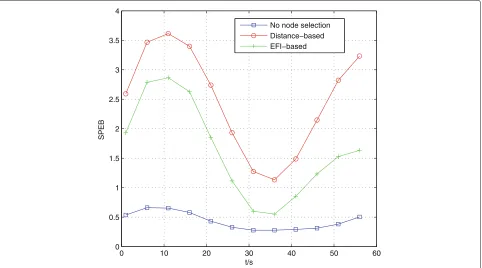
We consider a moving target, a network composed of 100 unknown nodes and 20 anchors. The 120 nodes are candidates. Unknown nodes are randomly distributed, and anchors are distributed uniformly. The trajectory of the target is an ellipse shown in Fig. 7. Figure 8 shows the SPEB of different neighbor selection algorithms. It should
0 1 2 3 4 5 6
1.15 1.2 1.25 1.3 1.35 1.4 1.45 1.5
Angle/(rad)
SPEB
Neighboring unknown node Neighboring anchor
0 10 20 30 40 50 60 70 80 90 100 0
10 20 30 40 50 60 70 80 90 100
x/m
y/m
Neighboring unknown nodes Neighboring anchor Moving target
Fig. 7Distribution of network nodes
be pointed out that the number of selected neighbors is the same for the two neighbor selection algorithms. Where blue line indicates cooperation without node selection, red indicates neighbor selection algorithm based on distance and green indicates neighbor selec-tion algorithm based on EFI. Obviously, node selecselec-tion
algorithm based on EFI can improve the positioning accuracy.
6 Conclusions
In this paper, we presented a new node selection algo-rithm based on EFI in wireless networks. Compared to
0 10 20 30 40 50 60
0 0.5 1 1.5 2 2.5 3 3.5 4
t/s
SPEB
No node selection Distance−based EFI−based
traditional algorithm, the proposed algorithm took into account power consumption and positioning accuracy simultaneously. Simulation results show that the proposed algorithm performs more effectively than the distance-based node selection algorithm. Since the position of a moving target at the adjacent time point is of great rele-vance, considering time-domain cooperative information to improve accuracy would be an interesting work in the future.
Acknowledgements
This work was supported by the National Science Foundation of China (61471077, 61301126) and the science and technology projects of Chongqing Municipal Education Commission (KJ1400413).
Competing interests
The authors declare that they have no competing interests.
Author details
1Chongqing Key Laboratory of Optical Communication and Networks, Chongqing University of Posts and Telecommunications, Chongwen Road, 400065 Chongqing, China.2School of Communication and Information engineering, Chongqing University of Posts and Telecommunications, Chongwen Road, 400065 Chongqing, China.
Received: 16 July 2016 Accepted: 6 October 2016
References
1. Z Xiong, F Sottile, MA Caceres, in2011 IEEE-APS Topical Conference on Antennas and Propagation in Wireless Communications. Hybrid WSN-RFID cooperative positioning based on extended Kalman filter (IEEE, Italy, 2011), pp. 990–993
2. SFA Shah, S Srirangarajan, AH Tewfik, Implementation of a directional beacon-based position location algorithm in a signal processing framework. IEEE Trans. Wireless Commun.9(3), 1044–1053 (2010) 3. W Dai, Y Shen, MZ Win, inWireless Communications and Networking
Conference (WCNC). Network navigation algorithms with power control (IEEE, New Orleans, 2015), pp. 1231–1236
4. W Dai, Y Shen, MZ Win, Energy-efficient network navigation algorithms. IEEE J. Selected Areas Commun.33(7), 1418–1430 (2015)
5. O Demigha, WK Hidouci, T Ahmed, On energy efficiency in collaborative target tracking in wireless sensor network: a review. IEEE Commun. Surv. Tutor.15(3), 1210–22 (2013)
6. MB Dai, F Sottile, MA Spirito, inIEEE 8th International Conference on Wireless and Mobile Computing, Network and Communications(WiMob). An energy efficient tracking algorithm in UWB-based sensor networks (IEEE, Spain, 2012), pp. 173–178
7. S Hadzic, J Rodriguez, inIndoor Positioning and Indoor Navigation (IPIN). Utility based node selection scheme for cooperative localization (IEEE, Portugal, 2011), pp. 1–6
8. HV Poor,An Introduction to Signal Detection and Estimation, 2nd edn. (Springer, New York, 1994)
9. I Reuven, H Messer, A Barankin-type lower bound on the estimation error of a hybrid parameter vector. IEEE Trans. Inform. Theory.43(3), 1084–1093 (1997)
10. Y Shen, MZ Win, inIEEE Wireless Communications and Networking Conference. Fundamental limits of wideband localization accuracy via Fisher information (IEEE, China, 2007), pp. 3046–3051
11. S Yuan, S Mazuelas, MZ Win, Network Navigation: Theory and Interpretation. IEEE J. Selected Areas Commun.30(9), 1823–1834 (2012) 12. MZ Win, A Conti, S Mazuelas, Network localization and navigation via
cooperation. IEEE Commun. Mag.49(5), 56–62 (2011)
13. S Yuan, MZ Win, Fundamental limits of wideband localization—part I: a general framework. IEEE Trans. Inform. Theory.56(10), 4956–4980 (2010) 14. Z Xiong, M Dai, F Sottile, MA Spirito, R Garello, inIEEE International
Conference on Communications. Cognitive and cooperative tracking approach in wireless networks (IEEE, Hungary, 2013), pp. 2717–2721
15. T Sathyan, M Hedley, inIEEE Trans. Mobile Comput. Fast and accurate cooperative tracking in wireless networks, (2013), pp. 1801–1813 16. Y Shen, H Wymeersch, MZ Win, Fundamental limits of wideband
localization: part II: cooperative networks. IEEE Trans. Inform. Theory. 56(10), 4981–5000 (2010)
Submit your manuscript to a
journal and benefi t from:
7Convenient online submission
7 Rigorous peer review
7Immediate publication on acceptance
7 Open access: articles freely available online
7High visibility within the fi eld
7 Retaining the copyright to your article