R E S E A R C H
Open Access
Wavelet multilevel augmentation method
for linear boundary value problems
Somlak Utudee
1and Montri Maleewong
2**Correspondence:
2Department of Mathematics,
Faculty of Science, Kasetsart University, Bangkok, 10900, Thailand Full list of author information is available at the end of the article
Abstract
This work presents a new approach to numerically solve the general linear two-point boundary value problems with Dirichlet boundary conditions. Multilevel bases from the anti-derivatives of the Daubechies wavelets are constructed in conjunction with the augmentation method. The accuracy of numerical solutions can be improved by increasing the number of basis levels, but the computational cost also increases drastically. The multilevel augmentation method can be applied to reduce the computational time by splitting the coefficient matrix into smaller submatrices. Then the unknown coefficients in the higher level can be solved separately. The
convergent rate of this method is 2s, where 1≤s≤p+ 1, when the anti-derivatives of the Daubechies wavelets orderpare applied. Some numerical examples are also presented to confirm our theoretical results.
MSC: 65J10; 65L10
Keywords: wavelets; multilevel augmentation method; boundary value problems;
Dirichlet boundary conditions
1 Introduction
Boundary value problems can be viewed as mathematical models in science and engineer-ing. For real world applications, exact solutions are not available. Numerical methods are required to solve numerically the models. The efficient methods provide approximate so-lutions by choosing the appropriate subspaces of solution spaces and their suitable bases. By applying suitable formulations, the linear model equation can be discretized to a linear system. A more accurate approximation can be obtained by increasing the number of basis functions. However, this leads to a larger discretized linear system. To save the computa-tional cost, one can use the multilevel augmentation method. The resulting coefficient matrix corresponding to the finer level of approximate spaces is obtained by augmenting a matrix corresponding to a coarser level. Instead of solving the linear system at the finer level, the coefficient matrix can be separated so that the smaller system at the coarser level can be taken. Thus, the additional computational cost is proportional to the dimension of the different space between the spaces of the finer level and the coarser level, not the di-mension of the whole finer level. This method allows us to develop faster and accurate algorithms for solving differential equations (see,e.g., [–], and []). These previous re-searches considered the second kind of equations and constructed piecewise polynomials as bases for the subspaces of the Sobolev spacesHm
(, ) consisting of elements satisfying
the homogeneous boundary conditions
u(j)() =u(j)() = , forj= , , . . . ,m– .
On the other hand, wavelets can be applied to discretize differential equations (see,e.g., [, ]). Related numerical methods with the applications of Haar and Legendre wavelets for solving boundary value problem are proposed by Siraj-ul-Islamet al.[, ]. The ad-vantage of wavelet basis is its capability to approximate solutions of differential equations. The wavelet Galerkin method is one of the most powerful methods that can be used to solve ordinary and partial differential equations (see,e.g., [–], and []). In addition, the accuracy of the approximate solutions can easily be improved by merely increasing the numbers of wavelet basis functions and the orders of wavelets. However, the wavelet basis is not straightforwardly adjusted to satisfy general boundary conditions. In , Xu and Shann introduced a different approach to handle the boundary conditions by using the anti-derivatives of Daubechies wavelets []. These anti-derivatives form bases for the finite-dimensional subspaces of Sobolev spaceHand are used to construct an algorithm
for approximating solutions.
In this work, we propose the method that combines the main advantages of wavelet bases and multilevel augmentation together. That is, we apply the multilevel augmentation of operators in conjunction with the anti-derivatives of Daubechies wavelets to approximate linear differential equations in the case of Dirichlet boundary conditions. The originality of this work is that we introduce the anti-derivatives of Daubechies wavelets for solving linear boundary value problems (see []) and apply this basis type with the augmenta-tion method proposed by Chen (see,e.g., [–] and []). By this concept, we obtain a new approach to reduce the computational time for solving the linear system resulting from discretizing a linear differential equation.
Given the intervalΩ:= (,R), we use the notationL(Ω) to denote the space of square integrable functions onΩwith standard inner product (·,·) defined by
(u,v) = R
u(x)v(x)dx
and the associated norm · .
LetHs(Ω) denote the standard Sobolev space with the norm ·
sgiven by
vs= s
i=
R
v(i)(x)dx.
According to the boundary condition, we work on the solution space
H(Ω) =v∈H(Ω)|v() =v(R) = ,
equipped with the inner product
[u,v] = R
and its associated norm|·|. It is well known that the norm|·|is equivalent to the standard norm · in this space.
Letp∈N. We will apply the multilevel augmentation method and anti-derivatives of wavelets of orderpto find numerical solutions of two-point boundary value problems with Dirichlet boundary conditions.
Assume that there exists a unique weak solutionu∈H
(Ω). To find numerical solutions,
we propose the following steps:
. The solution spaceH(Ω)is decomposed into orthogonal direct sum of subspaces. The anti-derivatives of the Daubechies wavelets are used to construct
finite-dimensional subspaces.
. Forn∈N, the multilevel method is applied to obtain thenth levelsolution by solving a linear system with matrix coefficients related to the anti-derivatives of the Daubechies wavelets.
. To obtain a solution at a higher level, namely(n+i)th level, the multilevel augmentation method is applied. By the algorithm to be presented, the
computational time for solving the linear system is reduced since the dimension of the matrix coefficient is smaller.
Finally, this work is organized as follows. Section gives an introduction to the anti-derivatives of the Daubechies wavelets and the finite-dimensional subspaces of the solu-tion spaceH
(Ω). In Section , we describe the algorithm to find approximate solutions
using the multilevel augmentation method. The optimal error estimates for the approxi-mate solutions are proven in Section , while some numerical examples are demonstrated in Section . Conclusions and future work are discussed in Section .
2 Bases for subspaces ofH1 0(
Ω
)In this section, we will introduce the wavelets of orderpand their anti-derivatives. These functions form orthonormal bases for the finite-dimensional subspacesSnof the solution spaceH
(Ω). More details can be found in [] and [].
To define the Daubechies wavelets, we consider two functions: thescaling functionφ(x) and thewavelet functionψ(x). The scaling function is obtained from the dilation equation. The wavelet function is defined from the scaling function. Details are described as follows.
Given a positive integerp, consider a sequence{ck}k∈Zsatisfying
ck= , fork∈ {/ , , , . . . , p– },
k ck= ,
k
(–)kkmck= , for ≤m≤p– ,
k
ckck–m= δm, for –p≤m≤p– .
The scaling functionφ(x) is the unique solution of the dilation equation
φ(x) =
p–
k=
ckφ(x–k),
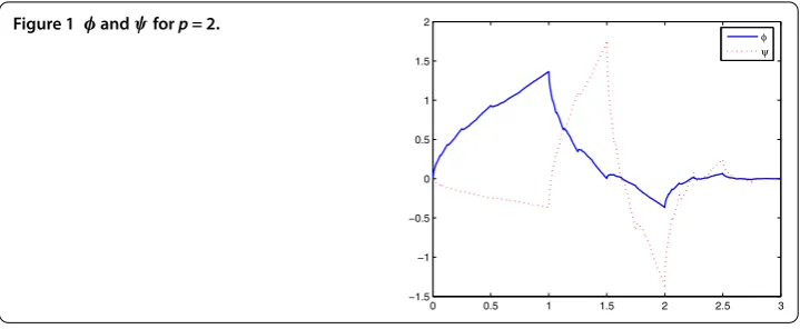
Figure 1 φandψforp= 2.
Let
ψ(x) =
p–
k=
(–)kcp––kφ(x–k).
The wavelet functionψ(x) is defined by
ψ(x) =ψ(x–p+ ).
The graphs ofφandψ forp= are shown in Figure . Define
ψjk(x) = ⎧ ⎨ ⎩
φ(x–k), j= –, √
jψ(jx–k), j≥.
The functionsψjk withj≥– and (j,k)∈Z×Zare calledwavelets of order p. It is well known that the set of wavelets forms an orthonormal basis forL(R).
Forj≥–, define the index setIjsuch that
k∈Ij ⇐⇒ ⎧ ⎨ ⎩
– p≤k≤p– , j= –,
– p≤k≤j(p– ) – , j≥.
{ψjk|Ω|j≥–,k∈Ij}is aframeofL(Ω). That is, thespan{ψjk|Ω|j≥–,k∈Ij} consist-ing of all linear expansions is equal toL(Ω).
Next, we define the anti-derivatives of wavelets satisfying the Dirichlet boundary con-dition, namely,
Ψjk(x) = x
ψjkds– x R
R
ψjkds, for ≤x≤R.
Forn∈N, we define a subspaceSnby
Sn=span{Ψjk|–≤j<n,k∈Ij}.
It is obvious that these subspaces are finite-dimensional subspaces ofH
(Ω) and they are
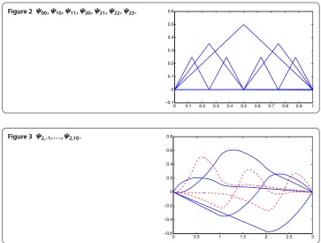
Figure 2 Ψ00,Ψ10,Ψ11,Ψ20,Ψ21,Ψ22,Ψ23.
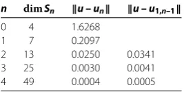
Figure 3 Ψ2,–1, . . . ,Ψ2,10.
need not be linearly independent. Xu and Shann [], introduced an index set Dj such that{Ψjk|–≤j<n,k∈Dj}is a basis forSn. The index setDjis defined by
k∈Dj ⇐⇒ ⎧ ⎨ ⎩
– p<k≤p– , j= –,
–p≤k≤j(p– ) –p, j≥.
Forp= , the basis functions{Ψjk|≤j<n,k∈Dj}forSnare the piecewise linear hier-archical basis functions with uniform mesh size,h= –n. The graphs ofΨ
,Ψ, . . . ,Ψ,
andΨare shown in Figure , while the graphs ofΨ,–, . . . ,Ψ,are shown in Figure .
It should be noted that the set
{Ψjk|≤j<n,k∈Dj}
is an orthonormal basis forSnwith the inner product [·,·] of the Sobolev spaceH (Ω) but
it is not orthonormal inL(Ω) when equipped with the standard inner product (·,·). Since
we require orthonormality inL(Ω) for our augmentation method, we apply the
Gram-Schmidt process to obtain an orthonormal basis forSnwith the standard inner product (·,·) inL(Ω). Thus, the set
{Ψjk|–≤j<n,k∈Dj}
is defined as orthonormal basis forSnin the present method.
3 Multilevel augmentation method algorithm
Letu∈H
(Ω) be the weak solution of a given differential equation. Suppose that the
variational form of the differential equation is
a(u,v) = (f,v), for allv∈H(Ω). ()
Let the approximate solutionunof the given equation be
un=
The main idea is to determine the coefficientsαjk in such a way thatunbehaves as if it were a weak solution onSn, that is,unsatisfies the linear system of equations,
a(un,Ψlm) = (f,Ψlm), for all –≤l<n,m∈Dj,
Letι: (j,k)→ibe the lexicographically enumerating function. That is,
ι(j,k)≤ι(l,m) ifj≤lorj=landk≤m.
We then obtain a linear system of the form Anun= fn, where Anis the coefficient matrix,
unis the unknown column vector, and fnis the column vector defined by
An=
The approximate solutionunobtained in this way is called thenth multilevel solutionof (). Next, we apply the augmentation method to approximate the next level solution,un+.
Suppose thatunis already solved. That is, the matrix representation unofunsatisfies the equation Anun= fn. We augment the matrix Anwith submatrices Bn, Cn, and Dnwhere
The coefficient matrix An+corresponding to the (n+ )st level is identified as
An+=
upper triangular matrix and a lower triangular matrix:
If the matrices Anand Dnare nonsingular, there exists a (unique) vector un,satisfying
augmentation solutionof (). The indexnrefers to theinitial level n, and refer to aone stepmethod to computeun+approximately. The linear system ofdimSn+can be solved
by considering two linear systems. One is the size ofdimSn, and another is the size of
dimSn+–dimSn= n(p– ).
In general, an approximationun,i+for (n+i+ )st multilevel solution is defined by setting
un,=un.
This completes the multilevel augmentation algorithm.
4 Error analysis
exists a positive constantCsuch that
u–un+ –nu–un≤C
–nsus, ≤s≤p+ .
In particular, if we consider separately the distance betweenuandunwith the standard Lnorm · , and the Sobolev norm ·
, we obtain
u–un ≤C
–nsus, ≤s≤p+ ,
u–un≤C
–ns–us, ≤s≤p+ .
The above estimations suggest that if we apply the wavelet of orderpandu∈H (Ω)∩
Hs(Ω), then the errors measured by the standard norm, and the Sobolev norm inL,
de-crease by the factors of p+, and p, respectively, fromnton+ level.
Next, we consider the distance between the solutionuand the (n+i)th multilevel aug-mentation solution, un,i, of (). In the remaining section, we denote byAthe operator corresponding to the matrix A, and we denote by u the column matrix representing ele-mentu.
Forn∈N, if the inverse operatorsA–n andD–n exist, then the (n+ )th multilevel aug-mentation solutionun,iexists. If there also exist anN∈N,α> , andδ> such that
A–
n≤α, Dn–≤δ, forn≥N,
and
lim
n→∞Bn=nlim→∞Cn= ,
the error for our method can be estimated as in the following theorem.
Theorem (Error for multilevel augmentation method) Let u∈H
(Ω)be the solution
of(). Suppose that there exist an N∈N, and positive constantsα andδ such that for n≥N the inverse operatorsA–
n ,D–n exist and
A–
n≤α, Dn–≤δ,
and
lim
n→∞Bn=nlim→∞Cn= .
If u∈H
(Ω)∩Hs(Ω),then there exist an M∈Nand positive constant csuch that,for
n≥M and i∈N∪ {},we have the estimate
u–un,i ≤c–(n+i)sus, ≤s≤p+ .
Proof By the hypotheses onA–
i∈N∪ {}. By Theorem . in [], there exists a positive constantCsuch that
Subtracting () from (), we have
An+i(un,i– un+i) =
Since An+iis nonsingular, we have the equation
From () and (), we conclude that
u–un,i ≤ u–un+i+un,i–un+i
≤C–(n+i)sus+ c
–(n+i)sus
≤
C+c
–(n+i)sus.
The above theorem suggests that, if the solutionu∈H
(Ω)∩Hs(Ω), and we apply the
multilevel augmentation method from leveln+i– ton+iby using the anti-derivatives wavelets of orderp, the errors measured in · decrease by a factor of p+. Thus the
behaviors of the decreasing error obtained by the multilevel, and the multilevel augmen-tation methods, are in the same order.
5 Examples
In this section, we illustrate the efficiency of the multilevel augmentation method in con-junction with the anti-derivatives of Daubechies wavelets of orderpto find the numerical solutions of the following boundary value problem:
–q(x)u+r(x)u=f(x), forx∈(,R), ()
with the Dirichlet conditions
u() =u(R) = ,
whereR= p– . It should be noted that the general interval (α,β) can be changed to (,R) by the method of changing variables.
We assume thatf ∈L(Ω), the coefficientsq andrare smooth in the closed interval
[,R] withq> andr≥. The variational form of () is
a(u,v) = (f,v), for allv∈H(Ω), ()
wherea(·,·) is the bilinear form defined by
a(u,v) = R
quv+ruv dx. ()
SinceA(·,·) is continuous and coercive onH
(Ω), by the Lax-Milgram lemma, there exists
a unique weak solutionu∈H(Ω) for ().
Note that we can also apply the multilevel augmentation method in conjunction with the anti-derivatives of the Daubechies wavelets orderpfor the cases with nonzero boundary conditions. For example, we consider the boundary value problem
with the boundary conditions
u(α) =c, u(β) =d.
We notice that the linear function
y(x) =βc–αd
β–α +
d–c
β–αx
satisfies the boundary conditions, that is,y(α) =candy(β) =d. Letu=y+wbe the weak solution of (). Sinceu(α) =candu(β) =d,w(α) =w(β) = . The variational form of the boundary value problem in this case is
a(w,v) = β
α
fv dx–a(y,v), for allv∈H(α,β), ()
wherea(·,·) is the bilinear form
a(w,v) = β
α
qwv+rwv dx. ()
Sincea(·,·) is continuous and coercive onH(α,β), by the Lax-Milgram lemma, there ex-ists a unique weak solutionw∈H(α,β) for ().
Example For the first example, we consider the two-point boundary value problem
–xu+xu=x–x– x+ , forx∈(, ), ()
with boundary conditionsu() =u() = .
The exact solution isu(x) =x–x. Here, we apply the Daubechies wavelets of order
p= to solve the problem. Numerical results for each level (n) are shown in Table . The column ofu–unpresents the numerical results obtained by the standard multilevel method. When increasing the level of approximations, the norm of theLerror decreases
by the factor of swhere ≤s≤. The numerical results by the multilevel augmentation method starting from the second and the third levels are shown in theu–u,n–and u–u,n–columns, respectively. At the same leveln, theLerrors are in the same order
as those of the standard multilevel method, except that its values are slightly greater. These additional errors come from the augmentation part which can be seen from the proof of Theorem . It can be seen further that the error from the augmentation method is getting closer to the error from the standard multilevel method asnbecomes large.
Example Consider the boundary value problem
–e–xu=πe–xcos(πx) +πsin(πx), forx∈(, ), ()
with boundary conditions,u() =u() = .
Table 1 Example 1: Numerical results forp= 1
Table 2 Example 2: Numerical results forp= 1
n dimSn u – un u – u1,n–1 u – u2,n–2 u – u3,n–3
2 3 1.6427
3 7 0.6045 0.6458
4 15 0.2424 0.2488 0.2494
5 31 0.1124 0.1162 0.1162 0.1170
6 63 0.0589 0.0607 0.0607 0.0606
7 127 0.0309 0.0325 0.0325 0.0325
8 255 0.0154 0.0161 0.0161 0.0161
9 511 0.0085 0.0087 0.0087 0.0087
Table 3 Example 2: Numerical results forp= 2
n dimSn u – un u – u1,n–1 well with the theoretical results. TheLerrors obtained by the multilevel augmentation
method starting from levels , , and are shown in the u–u,n–, u–u,n–, and u–u,n–columns, respectively. Their values are in the same order as the multilevel
method.
To apply the Daubechies wavelets of orderp= , we change the interval [, ] to [, ]. So we obtain the following boundary value problem:
–e–xu=π basis of orderp= are shown in Table . The rate ofLerror convergence is faster than
that of the casep= . Here, theL error is four times smaller than that of the previous
error level. This agrees with the theoretical result that theLerror should decrease by a
factor of s, where ≤s≤.
Example Consider the boundary value problem with nonzero boundary conditions
u–u=x– x+ , forx∈(, ), ()
Table 4 Example 3: Numerical results forp= 1
n dimSn u – un u – u1,n–1 u – u2,n–2 u – u3,n–3
2 3 0.4221
3 7 0.1993 0.2123
4 15 0.0994 0.1051 0.1049
5 31 0.0502 0.0561 0.0555 0.0555
6 63 0.0278 0.0303 0.0303 0.0302
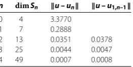
Table 5 Example 3: Numerical results forp= 2
n dimSn u – un u – u1,n–1
0 4 3.3770
1 7 0.2888
2 13 0.0351 0.0378
3 25 0.0044 0.0047
4 49 0.0007 0.0008
The exact solution isu= –x +x+x+ex–e+
(e–) . Numerical results forp= are shown
in Table . Column ofu–unpresents the numerical results obtained by the multilevel method. TheLerror is twice smaller than that of the previous error level, and agrees well with the theoretical results. TheLerrors obtained by the multilevel augmentation
method starting from levels , , , and are shown in theu–u,n–,u–u,n–, and u–u,n–columns, respectively. Their values are in the same order as the multilevel
method.
Numerical results from the wavelet basis of orderp= are shown in Table . The rate of Lerror convergence is faster than that of the casep= . Here, theLerrors is eight times smaller than that of the previous error level.
6 Conclusions
This present work is our attempt to apply the multilevel augmentation method using the anti-derivatives of Daubechies wavelets for approximating two-point boundary value problems with Dirichlet boundary conditions. This method is extended from the multi-level augmentation method that uses polynomial wavelet basis. An error analysis has also been presented. The rate of convergence is by a factor of s, ≤s≤p+ , wherepis the Daubechies wavelet order. At the same level, theLerror of the multilevel augmentation method is greater than that of the multilevel method, but they are in the same order.
The difficulty of this approach is that the anti-derivatives of Daubechies wavelet cannot be expressed in explicit form. One is required to solve the dilation equation to obtain a wavelet basis in an implicit formula. Here, we have done this using a numerical approxima-tion to obtain the basis funcapproxima-tion point by point. Also, it is not easy to extend this approach to problems in higher dimension.
Competing interests
The authors declare that they have no competing interests.
Authors’ contributions
All authors contributed equally to the writing of this paper. All authors read and approved the final manuscript.
Author details
1Department of Mathematics, Faculty of Science, Chiang Mai University, Chiang Mai, 50200, Thailand.2Department of
Mathematics, Faculty of Science, Kasetsart University, Bangkok, 10900, Thailand.
Acknowledgements
This research was supported by Chiang Mai University.
Received: 25 September 2014 Accepted: 8 April 2015 References
1. Chen, Z, Micchelli, CA, Xu, Y: A multilevel method for solving operator equations. J. Math. Anal. Appl.262, 688-699 (2001)
2. Chen, Z, Wu, B, Xu, Y: Multilevel augmentation methods for differential equations. Adv. Comput. Math.24(1-4), 213-238 (2006)
3. Chen, Z, Wu, B, Xu, Y: Multilevel augmentation methods for solving operator equations. Numer. Math. J. Chin. Univ.
14, 31-55 (2006)
4. Chen, Z, Xu, Y, Yang, H: Multilevel augmentation methods for solving ill-posed operator equations. Inverse Probl.22, 155-174 (2006)
5. Daubechies, I: Orthonormal bases of compactly supported wavelets. Commun. Pure Appl. Math.41, 909-996 (1988) 6. Glowinski, R, Lawton, W, Ravachol, M, Tenenbaum, E: Wavelet Solutions of Linear and Nonlinear Elliptic, Parabolic and
Hyperbolic Problems in One Space Dimension. Computing Methods in Applied Sciences and Engineering, pp. 55-120. SIAM, Philadelphia (1990)
7. Siraj-ul-Islam, Aziz, I, Al-Fahid, AS, Shah, A: A numerical assessment of parabolic partial differential equations using Haar and Legendre wavelets. Appl. Math. Model.37, 9455-9481 (2013)
8. Siraj-ul-Islam, Aziz, I, Sarler, B: The numerical solution of second-order boundary value problems by collocation with Haar wavelets. Math. Comput. Model.52, 1577-1590 (2010)
9. Amaratunga, K, Williams, JR, Qian, S, Weiss, J: Wavelet-Galerkin solutions for one dimensional partial differential equations, IESL Technical report, 9205, 2703-2716 (1994)
10. Jianhua, S, Xuming, Y, Biquan, Y, Yuantong, S: Wavelet-Galerkin solutions for differential equations. Wuhan Univ. J. Nat. Sci.3(4), 403-406 (1998)
11. Mishra, V, Sabina: Wavelet Galerkin solutions of ordinary differential equations. Int. J. Math. Anal.5(9), 407-424 (2011) 12. Qian, S, Weiss, J: Wavelets and the numerical solution of boundary value problems. Appl. Math. Lett.6(1), 47-52 (1993) 13. Xu, JC, Shann, WC: Galerkin-wavelet methods for two point boundary value problems. Numer. Math.63, 123-144