R E S E A R C H
Open Access
Exact spatiotemporal soliton solutions to
the generalized three-dimensional nonlinear
Schrödinger equation in optical fiber
communication
Xiaoli Wang
1*and Jie Yang
2*Correspondence: [email protected] 1School of Science, Qilu University
of Technology, Daxue Road, Jinan, 250353, China
Full list of author information is available at the end of the article
Abstract
In this paper, the exact spatiotemporal soliton solutions of the generalized (3 + 1)-dimensional nonlinear Schrödinger equation with varying coefficients in optical fiber communication are obtained explicitly by using the similarity transformation. In addition, the propagation characteristics of the spatiotemporal optical solitons which can be dramatically affected by the complicated group velocity dispersion and self-phase modulation are discussed in detail.
MSC: 35Q55; 35Q60; 35D99
Keywords: nonlinear Schrödinger equation; solitary wave; spatiotemporal soliton; similarity transformations
1 Introduction
The nonlinear Schrödinger (NLS) equation is one of the important mathematical mod-els in many fields of physics, which has been widely applied in Bose-Einstein condensates [–], nonlinear optical fiber communication [, ], plasma physics [, ], hydrodynamics [], and so on. Recently more and more people have been devoted to solving the exact solutions of the generalized NLS models [–]. Today, the temporal optical solitons of the NLS equation have been the objects of theoretical and experimental studies in opti-cal fiber communication, and optiopti-cal solitons are regarded as an important alternative to the next generation of ultrafast optical telecommunication systems. The study of optical solitons has reached the stage of a real-life application. The propagation of optical pulse in monomode optical fiber is governed by the NLS equation.
As is known to all, there are many kinds of powerful methods to obtain the exact solu-tions of various nonlinear wave equasolu-tions such as the NLS-type equasolu-tions. For example, inverse scattering method [], Bäcklund transformation [, ], Darboux transforma-tion [], Hirota bilinear method [, ], Lie symmetry method [, ], Riemann-Hilbert formulation [], generalized sine-cosine method [], similarity transformation [– ], multiple exp-function method [], and other efficient techniques [–]. Among all these methods, the similarity transformation is a powerful approach to solve high-dimensional and variable-coefficient NLS-type equations. In the framework of similarity
transformation, the high-dimensional and variable-coefficient NLS-type equations can be transformed into ordinary differential equations with constant coefficient, which are easy to be solved. Thus in this paper, with the aid of the symbolic computation, we use the sim-ilarity transformation and construct the analytical spatiotemporal soliton solutions to the generalized ( + )-dimensional nonlinear Schrödinger equation with varying coefficients in nonlinear optics
i∂u
∂z +β(z)∇
u+α(z, r)u+χ(z)|u|u=iγ(z)u, ()
where u≡u(z, r) with r = (x,y,t)∈ R, denotes the normalized slowly varying
com-plex wave packet envelope in a diffractive nonlinear Kerr medium with anomalous dis-persion, and |u| is the optical power. Notation ∇ ≡(∂
x,∂y,∂t) is a gradient operator,
and ∇ =∂x +∂y+∂t represents the D Laplacian. Here z is the normalized propa-gation distance, andt is the normalized retarded time,i.e., time in the frame of refer-ence moving with the wave packet. All coordinates are made dimensionless by the choice of coefficients. The real functionα(z, r) = rA(z)r stands for the linear potential, where
A(z) =diag(a(z),a(z),a(z)) is a diagonalz-dependent × matrix. The real functions
β(z),χ(z) andγ(z) stand for the group velocity dispersion (GVD), self-phase modulation (SPM) and linear gain (γ > ) or loss (γ < ), respectively. Strong interference of the effects of nonlinearity and varying dispersion can lead to a rich variety of possible configurations for dispersion management.
The generalized ( + )-dimensional nonlinear Schrödinger equation Eq. () is of con-siderable importance in optical fiber communication as it describes the amplification or absorption of pulses propagating in a monomode optical fiber with distributed dispersion and nonlinearity. In practical applications, the model is of primary interest not only for the amplification and compression of optical solitons in inhomogeneous systems, but also for the stable transmission of soliton control.
The paper is organized as follows. In Section , the similarity transformation is de-scribed, which converts a partial differential equation with variable coefficients into a family of first-order ordinary differential equations. In Section , several periodic trav-eling wave solutions are derived and some examples, which demonstrate the propagation characteristics of the spatiotemporal solitons, are given. Finally, a short conclusion is pre-sented.
2 Similarity transformation
Our goal is to search for a transformation connecting solutions of Eq. () with those of the stationary NLS equation with constant coefficients
Fξ ξ–qF– qF= . ()
Here,F≡F(ξ) is a function of the only variableξ≡ξ(z, r) whose relation to the original variables (z, r) is to be determined. Table shows a part of the Jacobi elliptic functions (JEFs) solutions of Eq. (). The constantsq andqappearing in Eq. () are related to
Table 1 Jacobi elliptic functions
Solution q2 q4 F
1 –(1 +M2) M2 sn
2 2M2– 1 –M2 cn
3 2 –M2 –1 dn
4 –(1 +M2) 1 ns
5 2M2– 1 1 –M2 nc
6 2 –M2 M2– 1 nd
7 2 –M2 1 –M2 sc
8 2M2– 1 –M2(1 –M2) sd
9 2 –M2 1 cs
10 –(1 +M2) M2 cd
11 2M2– 1 1 ds
12 –(1 +M2) 1 dc
13 M2/2 – 1 M4/4 sn/(1 +dn)
14 M2/2 – 1 M4/4 cn/(√1 –M2+dn)
i.e., sn(x)→sin(x), cn(x)→cos(x), dn(x)→,etc., and the periodic traveling wave solu-tions become the periodic trigonometric solusolu-tions. WhenM→, JEFs degenerate into hyperbolic functions,i.e., sn(x)→tanh(x), cn(x)→sech(x), dn(x)→sech(x),etc., and the periodic traveling wave solutions become the soliton solutions.
We consider the general similarity transformation
u(z, r) =f(z, r)Fξ(z, r)eiB(z,r), () wheref(z, r),B(z, r) andξ(z, r) are all real-valued functions to be determined.
RequiringF(ξ) to satisfy Eq. () andu(z, r) to be a solution of Eq. (), we substitute the ansatz () into Eq. () and after simple algebra obtain the set of equations
χf+ qβ|∇ξ|= , ()
fα+fβq|∇ξ|–|∇B|
+β∇f–fBz= , ()
fz+ β∇ ·f∇B– fγ = , ()
∇ ·f∇ξ= , ()
ξz+ β∇B· ∇ξ= . ()
To solve Eqs. ()-() explicitly, we first consider the special case off(z, r) depending only on the propagation coordinatez,i.e.,f(z, r)≡f(z). Then Eqs. ()-() are simplified
χf+ qβ|∇ξ|= , ()
α+βq|∇ξ|–|∇B|
–Bz= , () fz+
β∇B–γf = , ()
∇ξ= , ()
ξz+ β∇B· ∇ξ= . ()
We considerξparameterizing moving plains
where k(z) = [k(z),k(z),k(z)]. The nontrivial phase now reads
of each term be separately equal to zero, we obtain a system of algebraic and first-order ordinary differential equations that the parameters must satisfy:
hj;z+ βhj –aj= , ()
By solving Eqs. ()-() self-consistently, one obtains a set of conditions on the coeffi-cients and parameters, necessary for Eq. () to have exact periodic wave solutions.
3 Analytical solutions and the propagation characteristics of the spatiotemporal solitons
As it is clear, Eq. () which is critical of Eqs. ()-() is a standard Riccati equation with varying coefficients. The case ofβ≡const has been studied in many papers (see, for ex-ample, [, ] and the references therein). In this paper, we concentrate on the case of
β=emz,a
j=sje–mz,j= , , , wherem,sj(j= , , ) are arbitrary nonzero constants, and
the following set of exact solutions is found:
Here, bj, kj (j= , , ),ω, c, f are all arbitrary constants, and hj, θj, ρj are as
fol-Incorporating these solutions back into Eq. (), we can obtain the general periodic trav-eling wave solutions to the generalized NLSE
u=f ·Fk(z)·r+ω(z)·ei(rH(z)r+b(z)·r+c(z)). ()
As long as one chooses the constants according to the relations listed in Table and substitutes the appropriateF(ξ) into Eq. (), one obtains the exact periodic traveling wave solutions to the generalized ( + )-dimensional NLSE.
As an example, we select the solutions , , , in Table and the parametersb
j =kj= f= (j= , , ),ω=c= ,γ =cos(z). According to the value of parameterhj, we list
two classes.
3.1 The parameterh0
j = 1 (j= 1, 2, 3)
Family Taking parametersm= .,sj= ., we can obtain the periodic wave
solu-tion
u=f(z)F
and the nonlinearity coefficient
Family Taking parametersm= –.,sj= ., we can obtain the periodic wave
solution
Family Taking parameters m= ., sj= –., we can obtain the periodic wave
The nonlinearity coefficient is of the form
χ= –qe.z–sin(z)(.z+ ). ()
The functionf is of the form
f = e
–.z+sin(z)
(.z+ )
. ()
Family Taking parametersm= –.,sj= –., we can obtain the periodic wave
solution
u=
e.z+sin(z)
(–.z+ )
F e
.zL
–.z+ – z
–.z+
eiB, ()
where
B=–.(–.z+ )r
e–.z(–.z+ ) +
e.zL
–.z+ +
(q– )z
–.z+ ,
L=x+y+t, r=x+y+z. The nonlinearity coefficient is of the form
χ= –qe–.z–sin(z)(–.z+ ). ()
The functionf is of the form
f = e
.z+sin(z)
(–.z+ )
. ()
Figures and show the profiles of the nonlinear parameterχand the functionf as a function ofzgiven by Eqs. ()-(), ()-(), ()-(), ()-(). The functionf has
Figure 2 The functionsχandfof (a) and (b) given by Eqs. (45) and (46), and (c) and (d) given by Eqs. (48) and (49).
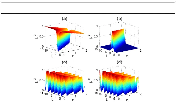
Figure 3 Density|u1|2as a function of propagation distanceL≡x+y+tandzgiven by Eq. (38), with
(a)F(ξ) = tanh(ξ), (b)F(ξ) = sech(ξ), (c)F(ξ) =sn(ξ),M= 0.5 and (d)F(ξ) =cn(ξ),M= 0.5.
an important effect on modulating the amplitude of the solutionu. It is seen in this situ-ation thatχandf are periodically oscillating along thez-axis. It can also be seen that the amplitude ofχincreases along thez-axis in Figure (a) and Figure (a), and the amplitude offdecreases along thez-axis in Figure (b) and Figure (b). However, the amplitude ofχ
decreases along thez-axis in Figure (c) and Figure (c), and the amplitude off increases along thez-axis in Figure (d) and Figure (d). Figure (a) and (b) presents the evolution plots of the dark and bright exact one-soliton solutionsugiven by Eq. () respectively
Figure 4 Density|u2|2as a function of propagation distanceL≡x+y+tandzgiven by Eq. (41), with
(a)F(ξ) = tanh(ξ), (b)F(ξ) = sech(ξ), (c)F(ξ) =sn(ξ),M= 0.5 and (d)F(ξ) =cn(ξ),M= 0.5.
Figure 5 Density|u3|2as a function of propagation distanceL≡x+y+tandzgiven by Eq. (44), with
(a)F(ξ) = tanh(ξ), (b)F(ξ) = sech(ξ), (c)F(ξ) =sn(ξ),M= 0.5 and (d)F(ξ) =cn(ξ),M= 0.5.
Eq. () under the strict integrable condition Eq. (). Figure shows the evolution plots of optical power|u|given by Eq. () under the strict integrable condition Eq. ().
Fig-ures and show the evolution plots of optical power|u|given by Eq. () under the
strict integrable condition Eq. (). Note thatF(ξ) in Figure is the solutions , in Table .
3.2 The parameterh0
j = 0 (j= 1, 2, 3)
Family Taking parametersm= .,sj= ., we can obtain the periodic wave
solu-tion as follows.
Case.
u=e–.z+sin(z)F
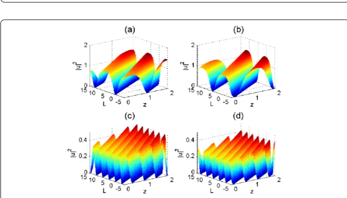
Figure 6 Density|u4|2as a function of propagation distanceL≡x+y+tandzgiven by Eq. (47), with
(a)F(ξ) = tanh(ξ), (b)F(ξ) = sech(ξ), (c)F(ξ) =sn(ξ),M= 0.5 and (d)F(ξ) =cn(ξ),M= 0.5.
Figure 7 Density|u4|2as a function of propagation distanceL≡x+y+tandzgiven by Eq. (47), with
(a)F(ξ) =sn/(1 +dn),M= 0.9999, (b)F(ξ) =cn/(√1 –M2+dn),M= 0.9999, (c)F(ξ) =sn/(1 +dn),
M= 0.5 and (d)F(ξ) =cn/(√1 –M2+dn),M= 0.5.
where
B= .e–.zr+e–.zL– (q– )
e–.z– ,
L=x+y+t, r=x+y+z. The nonlinearity coefficient is of the form
χ= –qe.z–sin(z).
Case.
u=e.z+sin(z)F
where
B= –.e–.zr+e.zL+ (q– )
e.z– ,
L=x+y+t, r=x+y+z. The nonlinearity coefficient is of the form
χ= –qe.z–sin(z).
Family Taking parameters m= –., sj= ., we can obtain the periodic wave
solution as follows.
Case.
u=e–.z+sin(z)F
e–.zL+ e–.z– eiB, where
B= .e.zr+e–.zL– (q– )
e–.z– ,
L=x+y+t, r=x+y+z. The nonlinearity coefficient is of the form
χ= –qe–.z–sin(z).
Case.
u=e.z+sin(z)F
e.zL– e.z– eiB, where
B= –.e.zr+e.zL+ (q– )
e.z– ,
L=x+y+t, r=x+y+z. The nonlinearity coefficient is of the form
χ= –qe–.z–sin(z).
Family Taking parameters m= ., sj= –., we can obtain the periodic wave
solution
u=e–.z+sin(z)F
e–.zL– zeiB, where
B= .e–.zr+e–.zL+ (q– )z,
The nonlinearity coefficient is of the form
χ= –qe.z–sin(z).
Family Taking parametersm= –.,sj= –., we can obtain the periodic wave
solution
u=e.z+sin(z)F
e.zL– zeiB, where
B= –.e.zr+e.zL+ (q– )z,
L=x+y+t, r=x+y+z. The nonlinearity coefficient is of the form
χ= –qe–.z–sin(z).
The evolution plots of solutionsuin Families - are very close to the evolution plots in [], and we omit the corresponding discussion for the limit of the length.
4 Conclusions
In conclusion, we have used similarity transformation to construct analytical spatiotem-poral soliton solutions of the generalized ( + )-dimensional NLS equation with varying coefficients, and also investigated the propagation characteristics of the spatiotemporal solitons which can be dramatically affected by the complicated potential.
Competing interests
The authors declare that they have no competing interests.
Authors’ contributions
All authors completed the paper together. All authors read and approved the final manuscript.
Author details
1School of Science, Qilu University of Technology, Daxue Road, Jinan, 250353, China.2School of Science, Beijing
Information Science and Technology University, Xiaoying East Road, Beijing, 100192, China.
Acknowledgements
This work is supported by the Science and Technology Project of Beijing Municipal Commission of Education (Grant No. KM201311232021).
Received: 16 September 2015 Accepted: 2 November 2015
References
1. Bradley, CC, Sackett, CA, Tollett, JJ, Hulet, RG: Evidence of Bose-Einstein condensation in an atomic gas with attractive interactions. Phys. Rev. Lett.27, 1687-1690 (1995)
2. Saito, H, Ueda, M: Dynamically stabilized bright solitons in a two-dimensional Bose-Einstein condensate. Phys. Rev. Lett.90, 040403 (2003)
3. Wang, DS, Hu, XH, Hu, J, Liu, WM: Quantized quasi-two-dimensional Bose-Einstein condensates with spatially modulated nonlinearity. Phys. Rev. A81, 025604 (2010)
4. Porsezian, K, Hasegawa, A, Serkin, VN, Belyaeva, TL, Ganapathy, R: Dispersion and nonlinear management for femtosecond optical solitons. Phys. Lett. A361, 504-508 (2007)
5. Calvo, GF, Belmonte-Beitia, J, Pérez-García, VM: Exact bright and dark spatial soliton solutions in saturable nonlinear media. Chaos Solitons Fractals41, 1791-1798 (2009)
6. Rose, HA, Weinstein, MI: On the bound states of the nonlinear Schrödinger equation with a linear potential. Physica D
7. Oelza, D, Trabelsi, S: Analysis of a relaxation scheme for a nonlinear Schrödinger equation occurring in plasma physics. Math. Model. Anal.19, 257-274 (2014)
8. Nore, C, Brachet, ME, Fauve, S: Numerical study of hydrodynamics using the nonlinear Schrödinger equation. Physica D65, 154-162 (1993)
9. Wang, DS, Hu, XH, Liu, WM: Localized nonlinear matter waves in two-component Bose-Einstein condensates with time-and space-modulated nonlinearities. Phys. Rev. A82, 023612 (2010)
10. Yan, ZY: Exact analytical solutions for the generalized non-integrable nonlinear Schrödinger equation with varying coefficients. Phys. Lett. A374, 4838-4843 (2010)
11. Wang, DS, Song, SW, Xiong, B, Liu, WM: Vortex states in rotating Bose-Einstein condensate with spatiotemporally modulated interaction. Phys. Rev. A84, 053607 (2011)
12. Ablowitz, MJ, Segur, H: Soliton and the Inverse Scattering Transformation. SIAM, Philadelphia (1981)
13. Rogers, C, Schief, WK: Backlund and Darboux Transformations: Geometry and Modern Applications in Soliton Theory. Cambridge University Press, Cambridge (2002)
14. Wang, DS, Wei, XQ: Integrability and exact solutions of a two-component Korteweg de Vries system. Appl. Math. Lett.
51, 60-67 (2016)
15. Matveev, VB, Salle, MA: Darboux Transformation and Solitons. Springer, Berlin (1991)
16. Hirota, R: Exact solution of the Korteweg de Vries equation for multiple collisions of solitons. Phys. Rev. Lett.27, 1192-1194 (1971)
17. Ma, WX: Generalized bilinear differential equations. Stud. Nonlinear Sci.2, 140-144 (2011)
18. Belmonte-Beitia, J, Pérez-García, VM, Vekslerchik, V: Lie symmetries and solitons in nonlinear systems with spatially inhomogeneous nonlinearities. Phys. Rev. Lett.98, 064102 (2007)
19. Ma, WX, Chen, M: Direct search for exact solutions to the nonlinear Schrödinger equation. Appl. Math. Comput.215, 2835-2842 (2009)
20. Wang, DS, Zhang, DJ, Yang, J: Integrable properties of the general coupled nonlinear Schrödinger equations. J. Math. Phys.51, 023510 (2010)
21. Yan, ZY: Envelope compactons and solitary patterns. Phys. Lett. A355, 212-215 (2006)
22. Belmonte-Beitia, J, Pérez-García, VM, Vekslerchik, V, Konotop, VV: Localized nonlinear waves in systems with time- and space-modulated nonlinearities. Phys. Rev. Lett.100, 164102 (2008)
23. Wang, DS, Shi, YR, Chow, KW, Yu, ZX, Li, XG: Matter-wave solitons in a spin-1 Bose-Einstein condensate with time-modulated external potential and scattering lengths. Eur. Phys. J. D67, 242 (2013)
24. Wang, DS, Ma, YQ, Li, XG: Prolongation structures and matter-wave solitons inF= 1 spinor Bose-Einstein condensate with time-dependent atomic scattering lengths in an expulsive harmonic potential. Commun. Nonlinear Sci. Numer. Simul.19, 3556-3569 (2014)
25. Ma, WX, Zhu, ZN: Solving the (3 + 1)-dimensional generalized KP and BKP equations by the multiple exp-function algorithm. Appl. Math. Comput.218, 11871-11879 (2012)
26. Ma, WX, Wu, HY, He, JS: Partial differential equations possessing Frobenius integrable decompositions. Phys. Lett. A
364, 29-32 (2007)
27. Yan, ZY: The new tri-function method to multiple exact solutions of nonlinear wave equations. Phys. Scr.78, 035001 (2008)
28. Wang, XL, Wu, ZH: New exact solutions and dynamics in (3 + 1)-dimensional Gross-Pitaevskii equation with repulsive harmonic potential. Commun. Theor. Phys.61, 583-589 (2014)
29. Ma, WX, Fuchssteiner, B: Explicit and exact solutions to a Kolmogorov-Petrovskii-Piskunov equation. Int. J. Non-Linear Mech.31, 329-338 (1996)