R E S E A R C H
Open Access
Dynamics of a single population system
with impulsively unilateral diffusion and
impulsive input toxins in polluted
environment
Shaohong Cai
1, Jianjun Jiao
1*and Limei Li
2*Correspondence:
1School of Mathematics and
Statistics, Guizhou Key Laboratory of Economic System Simulation, Guizhou University of Finance and Economics, Guiyang, 550004, P.R. China
Full list of author information is available at the end of the article
Abstract
In this paper, we consider a single population system with impulsively unilateral diffusion and impulsive input toxins in a polluted environment. All solutions of the investigated system are proved to be uniformly bounded. By mathematical analysis methods and the theory of impulsive differential equations, the condition of the glob-ally asymptoticglob-ally stable population-extinction solution of the investigated system is obtained. The permanent condition of the investigated system is also obtained. Finally, numerical analysis is carried out to illustrate our results. Our results provide a reliable theory basis for exploring biological resource management in a polluted environment.
Keywords: population system; impulsively unilateral diffusion; polluted environment; extinction; permanence
1 Introduction
Dispersal is a ubiquitous phenomenon in the natural world. It is important for us to under-stand the ecological and evolutionary dynamics of populations mirrored by the large num-ber of mathematical models devoting to it in the scientific literature [–]. In recent years, the analysis of these models focus on the coexistence of population and local (or global) stability of equilibria [, ]. Spatial factors play a fundamental role on the persistence and stability of the population, and the complete results have not yet been obtained even in the simplest one-species case. Most previous papers focused on the population dynamical system modeled by the ordinary differential equations. But in practice, it is often the case that diffusion occurs in regular pulses. For example, when winter comes, birds will migrate between patches in search for a better environment, whereas they do not diffuse in other seasons, and the excursion of foliage seeds to occur at fixed periods of time every year, thus impulsive diffusion provides a more natural description. Jiaoet al.[] presented a delayed predator-prey model with impulsive diffusion between two patches. They obtained the permanent condition of the system by the theory of impulsive delay differential equation. The most threatening problem to society is the change in both terrestrial and aquatic environment caused by the different kinds of stresses (temperature, toxicants/pollutants, etc.) affecting the long term survival of species, human life, and biodiversity of the
tat [–]. The presence of a toxicant in the environments decreases the growth rate of species and its carrying capacity. In recent years, some investigations have been carried out to study the effect of toxicant on a single species population [–], and a lot of scholars have adopted a mathematical modeling approach to study the influence of environmental pollution on the surviving of a biological population [, ]. Most of the previous work assumed that input of toxicant was continuous. The toxicants, however, are often emitted to the environment with regular pulse []. A lot of data have indicated that the use of agriculture chemicals may cause potential harm to the health of both human beings and other living beings. If the spraying of agriculture chemicals can be regarded as time pulse discharge, modeling by the continuous input of toxin can be regarded as obsolete and should be replaced by impulsive perturbations. In this case, though the discharge of toxin is transient, the influence of the toxin will last long. Therefore, it is very important how to control the pulse input cycle of toxin to protect the population’s persistent existence.
Theories of impulsive differential equations have been introduced into population dy-namics lately [–]. Impulsive equations are found in almost every domain of applied science and have been studied in many investigations [–], they generally describe phenomena which are subject to steep or instantaneous changes. Especially, Jiao et al. [] suggested releasing pesticides is combined with transmitting infective pests into an SI model. This may be accomplished by avoiding periods when the infective pests would be exposed or placing the pesticides in a location where the transmitting infective pests would not contact it. So we address an impulsive differential equation modeling the pro-cess of releasing infective pests and spraying pesticides at different fixed moments.
The organization of this paper is as follows. In the next section, we introduce the model and background concepts. In Section , some important lemmas are presented. In Sec-tion , we give the globally asymptotically stable condiSec-tion of populaSec-tion-extincSec-tion solu-tion of system (.) and the populasolu-tion permanent condisolu-tion of system (.). In Secsolu-tion , a numerical analysis and a brief discussion are given.
2 The model
In this work, we consider a single population system with impulsively unilateral diffusion and impulsive input toxins in a polluted environment,
where we suppose that system (.) is composed of two patches connected by diffusion. Patch is occupied by populationx(t). Patch is occupied by populationy(t).x(t) rep-resents the density of the population at patch , andy(t) represents the density of the population at patch . Patch is polluted periodically. There is no pollution in patch . co(t) represents the concentration of toxicant in the organism of the population at timet in patch .ce(t) represents the concentration of the toxicant in the system environment of patch . The intrinsic rate of natural increase and density dependence rate of the popula-tion in the first habitat are denoted bya,b, respectively.a/bdenotes the carrying capacity of population in the patch .d> represents the death rate of the population in patch . fce(t) is the organism’s net uptake of toxicant from the system environment at timetin patch . –gc(t) and –mc(t) represent the elimination and depuration rates of toxicant in
the organism at timetin patch , respectively. –hce(t) represents the totality of losses from the system environment including processes such as biological transformation, chemical hydrolysis, volatilization, microbial degradation, and photosynthetic degradation at timet in patch , andh>fis assumed in this paper.β> represents the depletion rate coefficient of the normal population during to the environment pollutant concentration of patch . The impulsive inputting toxicant occurs everyτperiod (τis a positive constant)in patch .
ce(t) =ce(t+) –ce(t).μ≥ represents the amount of the pulse input of toxicant concen-tration att= (n+l)τ, <l< ,n∈Z+in patch .Dis the dispersal rate between the two
patches. It is assumed that the net exchange from patch to patch is proportional to the pollution degree of patch . The pulse diffusion occurs everyτperiod (τ is a positive con-stant), the system evolves from its initial state without being further affected by diffusion until the next pulse appears, wherex(nτ) =x(nτ+) –x(nτ).x(nτ+) represents the density of the population in patch immediately after thenth diffusion pulse at timet=nτ, while x(nτ) represents the density of the population in patch before thenth diffusion pulse at timet=nτ,n= , , , . . . .
In this paper, we always assume that
(A) the population diffuses periodically from patch to patch for dodging polluted environment in patch ;
(A) the toxicants are emitted to the environment with regular pulse in patch , and patch has no pollution.
3 Preliminary lemmas
Before discussing the main results, we will give some definitions, notations, and lemmas. Denote byf = (f,f,f,f) the map defined by the right hand of system (.). The solution
of system (.), denoted byz(t) = (x(t),y(t),co(t),ce(t))T, is a piecewise continuous function z:R+→R+, whereR+= [,∞),R+={z∈R:z> }.z(t) is continuous on (nτ, (n+l)τ] and
((n+l)τ, (n+)τ] (n∈Z+, ≤l≤). According to [], the global existence and uniqueness
of solutions of system (.) is guaranteed by the smoothness properties off, which denotes the mapping defined by the right-hand side of system (.).
LetV:R+×R+→R+, thenV is said to belong to classV, if
(i) Vis continuous in(nτ, (n+l)τ]×R+and((n+l)τ, (n+ )τ]×R+, for eachz∈R+,
n∈Z+.lim(t,u)→((n+l)τ+,z)V(t,u) =V((n+l)τ+,z), and
lim(t,u)→((n+)τ+,z)V(t,u) =V((n+ )τ+,z)exist;
Definition . IfV∈V, then for (t,z)∈(nτ, (n+l)τ]×R+and ((n+l)τ, (n+ )τ]×R+,
the upper right derivative ofV(t,z) with respect to the impulsive differential system (.) is defined as
D+V(t,z) =lim h→sup
h V
t+h,z+hf(t,z)–V(t,z).
Now, we show that all solutions of system (.) are uniformly ultimately bounded.
Lemma . There exists a constant M> such that x(t)≤M,y(t)≤M and co(t)≤M, ce(t)≤M for each solution(x(t),y(t),co(t),ce(t))of system(.)with all t large enough. Proof DefineV(t) =x(t) +y(t) +co(t) +ce(t), and chooseλ=min{d,g+m,h–f}, thent=nτ, we have
D+V(t) +λV(t)
≤x(t) (a+λ) –bx(t)– (d–λ)y(t) – (g+m–λ)co(t) – (h–f–λ)ce(t)
< –b
x(t) – a+λ b
+(a+λ)
b < (a+λ)
b .
For convenience, we denoteζ=(a+λb). Whent= (n+l)τ,
V(n+l)τ+=x(n+l)τ+y(n+l)τ+co
(n+l)τ+ce
(n+l)τ+μ≤V(n+l)τ+μ.
Whent= (n+ )τ,
V(n+ )τ+=x(n+ )τ+y(n+ )τ+co
(n+ )τ+ce
(n+ )τ–Dx(t) +Dx(t)
=V(n+ )τ.
From Lemma . [], page , fort∈(nτ, (n+l)τ] and ((n+l)τ, (n+ )τ], we have
V(t)≤V+e–dt+ζ d
–e–dt+μe –d(t–τ)
–e–dτ +ξ edτ edτ– →
ζ
d+μ edτ
edτ– , ast→ ∞. SoV(t) is uniformly ultimately bounded. Hence, by the definition ofV(t), there exists a constantM> such thatx(t)≤M,y(t)≤M,co(t)≤M, andce(t)≤Mfortlarge enough.
The proof is complete.
The subsystem of (.) is
⎧ ⎪ ⎪ ⎪ ⎪ ⎨ ⎪ ⎪ ⎪ ⎪ ⎩
dco(t)
dt =fce(t) – (g+m)co(t), dce(t)
dt = –hce(t),
t=nτ,n∈Z+,
co(t) = ,
ce(t) =μ,
t=nτ,n∈Z+.
(.)
Lemma .[] System(.)has a unique positiveτ-periodic solution(co(t),ce(t)),which is globally asymptotically stable,where
⎧
In this section, we firstly prove that system (.) is permanent. For system (.) obviously exists a population-extinction boundary periodic solution (, ,co(t),ce(t)). Then we prove that the population-extinction boundary periodic solution (, ,co(t),ce(t)) of system (.) is globally asymptotically stable.
4.1 The permanence of (2.1)
The subsystem of system (.) is obtained as follows:
⎧
Considering the first equation of system (.) and Remark ., we have
x(t) a–β(Mo+ε) –bx(t)
Then we can obtain two comparative systems, referring to system (.),
It is clear that
We can easily obtain the analytic solution of system (.) between pulses,i.e. ⎧
Considering the third and fourth equations of system (.), we have the stroboscopic map of system (.),
Proof For convenience, we denote (xn+l
,yn+l) = (x((n+l)τ+),y((n+l)τ+)). The linear form
ofMbeing less than . IfMsatisfies theJurycriteria [], we can know the eigenvalue of Mless than , we have
–trM+detM> . (.)
(i) If ( –D)ae(a–βMo)τ <a–βM
o, there must exist a sufficiently smallε> such that ( –D)ae(a–β(Mo+ε))τ <a–β(M
of system (.), we have
M= ⎛ ⎝(–D)ae
(a–β(Mo+ε))τ
a–β(Mo+ε)
Dae(a–β(Mo+ε))τ a–β(Mo+ε) e
–dτ ⎞
⎠. (.)
Then
–trM+detM= –
( –D)ae(a–β(Mo+ε))τ a–β(Mo+ε)
+e–dτ
+
( –D)ae(a–β(Mo+ε))τ a–β(Mo+ε) ×
e–dτ
=
( –D)e(a–βMo)τ a–β(Mo+ε)
–
×e–dτ–
=
( –D)e(a–βMo)τ– (a–β(M o+ε)) a–β(Mo+ε)
×e–dτ– > .
From theJurycriteria,G(, ) is locally stable, then it is globally asymptotically stable.
(ii) If ( –D)ae(a–βMo)τ >a–βM
o, there must exist a sufficiently smallε> such that ( –D)ae(a–β(Mo+ε))τ >a–β(M
o+ε), ThenG(, ) is unstable.G(x∗,y∗) exists, and
M=
(–D)AB
(B+Cx∗)
DAB
(B+Cx∗) E
, (.)
whereA=ae(a–β(Mo+ε))τ,B=a–β(M
o+ε),C=b[e(a–β(Mo+ε))τ– ],E=e–dτ, and <E< . Then
–trM+detM= –
( –D)AB (B+Cx∗) +E
+( –D)AB (B+Cx∗) ×E
=
( –D)AB (B+Cx∗)–
×(E– )
=a–β(Mo+ε) – ( –D)ae
(a–β(Mo+ε))τ
( –D)ae(a–β(Mo+ε))τ ×(E– ) >
and from theJurycriteria,G(x∗,y∗) is locally stable, and then it is globally asymptotically
stable. This completes the proof.
Similarly to the methods in [], the following lemma can easily be proved.
Theorem . (i) If
( –D)ae(a–βMo)τ <a–βM o,
the triviality periodic solution(, )of system(.)is globally asymptotically stable. (ii) If
( –D)ae(a–βMo)τ
the periodic solution(x(t),y(t))of system(.)is globally asymptotically stable,
where ⎧ ⎨ ⎩
x(t) =
ae(a–β(Mo+ε))(t–(n+l)τ)x∗
(a–β(Mo+ε))+b[e(a–β(Mo+ε))(t–(n+l)τ)–]x∗
, (n+l)
τ<t≤(n+l+ )τ,
y(t) =y∗e–d(t–(n+l)τ), (n+l)τ<t≤(n+l+ )τ,
(.)
wherex∗ andy∗ are determined as in(.).
From Theorem ., we can obtain the following.
Remark . If ( –D)ae(a–βMo)τ >a–βM
o, for any sufficiently smallε> , there exists a
Tsuch thatx(t)≥x(t) –εandy(t)≥y(t) –εfort>T.
We can also obtain the analytic solution of system (.) between pulses,i.e. ⎧
⎨ ⎩
x(t) = ae
(a–β(mo–ε))(t–(n+l)τ)x ((n+l)τ+)
(a–β(mo–ε))+b[e(a–β(mo–ε))(t–(n+l)τ)–]x
((n+l)τ+), (n+l)τ<t≤(n+l+ )τ,
y(t) =y((n+l)τ+)e–d(t–(n+l)τ), (n+l)τ<t≤(n+l+ )τ.
(.)
Considering the third and fourth equations of system (.), we have the stroboscopic map of system (.),
⎧ ⎨ ⎩
x((n+l+ )τ+) = ( –D) ae
(a–β(mo–ε))τx ((n+l)τ+)
(a–β(mo–ε))+b[e(a–β(mo–ε))τ–]x((n+l)τ+),
y((n+l+ )τ+) =D ae
(a–β(mo–ε))τx ((n+l)τ+) (a–β(mo–ε))+b[e(a–β(mo–ε))τ–]x
((n+l)τ+)+e –dτy
((n+l)τ+).
(.)
The two fixed points of (.) are obtained asG(, ) andG(x∗,y∗), where
⎧ ⎪ ⎪ ⎪ ⎪ ⎪ ⎨ ⎪ ⎪ ⎪ ⎪ ⎪ ⎩
x∗=(–D)ae(a–β(mo–ε))τ–[a–β(mo–ε)]
b(e(a–β(mo–ε))τ–) ,
( –D)ae(a–β(mo–ε))τ >a–β(m o–ε), y∗=De(a–β(mo–ε))τ[(–D)ae(a–β(mo–ε))τ–(a–β(mo–ε))]
(–D)be(a–β(mo–ε))τ(e(a–β(mo–ε))τ–)(–e–dτ) ,
( –D)ae(a–β(mo–ε))τ >a–β(m o–ε).
(.)
Similarly to system (.), we have some theorems as regards system (.).
Theorem . (i) If
( –D)ae(a–β(mo–ε))τ<
a–β(mo–ε),
the fixed pointG(, )of(.)is globally asymptotically stable. (ii) If
( –D)ae(a–β(mo–ε))τ
>a–β(mo–ε),
the fixed pointG(x∗,y∗)of(.)is globally asymptotically stable.
Theorem .
(i) If( –D)ae(a–β(mo–ε))τ <a–β(m
o–ε),the triviality periodic solution(, )of system
(ii) If( –D)ae(a–β(mo–ε))τ >a–β(m
o–ε)the periodic solution(x(t),y(t))of system (.)is globally asymptotically stable,where
⎧ ⎨ ⎩
x(t) = ae
(a–β(mo–ε))(t–(n+l)τ)x∗
(a–β(mo–ε))+b[e(a–β(mo–ε))(t–(n+l)τ)–]x∗
, (n+l)τ <t≤(n+l+ )τ,
y(t) =y∗e–d(t–(n+l)τ), (n+l)τ <t≤(n+l+ )τ.
(.)
Herex∗andy∗are determined as in(.).
Remark . If ( –D)ae(a–β(mo–ε))τ<a–β(m
o–ε), for any sufficiently smallε> , there
exists aTsuch thatx(t)≤εandy(t)≤εfort>T.
From Theorem ., Remark ., Theorem ., and Remark ., we present an important theorem in this paper.
Theorem . (i) If
( –D)ae(a–βmo)τ <a–βm o
holds,the population of system(.)will go extinct. (ii) If
( –D)ae(a–βMo)τ
>a–βMo
holds,the population of system(.)is permanent.
Proof (i) According to the impulsive comparative theorem [] and the condition ( – D)ae(a–βmo)τ<a–βm
o, there exists a sufficiently smallε> such that ( –D)ae(a–β(mo–ε))τ < a–β(mo–ε), and, from Remark ., for any sufficiently smallε> , there exists aT>
such thatx(t)≤x(t)≤εandy(t)≤y(t)≤εfort>T. That is to say, for any sufficiently
smallε> , there exists aT> such thatx(t)≤εandy(t)≤εfort>T. These show
that the population of system (.) will go extinct.
(ii) According to the impulsive comparative theorem [] and the condition ( – D)ae(a–βMo)τ>a–βM
o, there exists a sufficiently smallε> such that (–D)ae(a–β(Mo+ε))τ> a–β(Mo+ε), and from Remark ., for any sufficiently smallε> , there exists aT>
such thatx(t)≥x(t)≥x(t) –ε≥x∗e–(d+Mo+ε)τ –ε
=mandy(t)≥y(t)≥y(t) –ε≥
y∗e–dτ –ε
=m fort>T, wherex∗ andy∗ are determined as (.). From Lemma .,
there existM> and T> such thatx(t) <Mandy(t) <Mfort>T. From the above discussion, we knowm<x(t) <Mandm<y(t) <Mfort>max{T,T}. That is to say, the
population of system (.) is permanent.
From Lemma ., Remark ., and Theorem ., we have the following.
Theorem . If
( –D)ae(a–βMo)τ >a–βM o,
4.2 The globally asymptotical stability of population-extinction boundary periodic solution of (2.1)
Theorem . If
( –D)ae(a–βmo)τ <a–βm o,
holds,the population-extinction boundary periodic solution(, ,co(t),ce(t))of system(.) is globally asymptotically stable,where mois defined as Remark..
Proof Firstly, we prove the local stability. Definex(t) =x(t),y(t) =y(t),z(t) =co(t) –co(t),
It is easy to obtain the fundamental solution matrix
(t) =
There is no need to calculate the exact form of†as it is not required in the analysis that follows. The linearization of the th, th, th, and th equations of system (.) is
⎛
The linearization of the th, th, th, and th equations of system (.) is
⎛
The stability of the population-extinction periodic solution (, ,co(t),ce(t)) is determined by the eigenvalues of
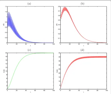
Figure 1 Globally asymptotically stable population-extinction periodic solution of system (2.1) with x(0) = 1,y(0) = 0.5,co(0) = 0.5,ce(0) = 0.5,a= 0.4,b= 1,d= 0.1,β= 0.05,μ= 2,f= 0.1,m= 0.1, g= 0.1,l= 0.25,D= 0.1,τ= 1. (a)Time-series ofx(t);(b)time-series ofy(t);(c)time-series ofco(t);
(d)time-series ofce(t).
which are
λ= ( –D)exp
τ
a–βc(s)
ds
,
λ=e–dτ < ,
λ=exp –(g+m)τ
< ,
and
λ=e–hτ < .
According the condition, we easily find ( –D)e(a–βmo)τ < . Then, from Remark ., we have ( –D)exp(τ(a–βco(s))ds) < , then λ < . From the Floquet theory [], the
population-extinction (, ,co(t),ce(t)) is locally stable.
The following task is to prove the global attraction. Then we have subsystem (.) of system (.). From Lemma ., we know that theτ-periodic solution (co(t),ce(t)) of system (.) has globally asymptotical stability, and
⎧ ⎨ ⎩
co(t)≥co(t) –ε≥mo–ε, ce(t)≥ce(t) –ε,
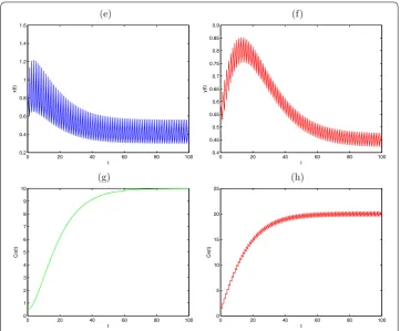
Figure 2 The permanence of system (2.1) withx(0) = 1,y(0) = 0.5,co(0) = 0.5,ce(0) = 0.5,a= 0.4,b= 1, d= 0.1,β= 0.05,μ= 1,f= 0.1,m= 0.1,g= 0.1,l= 0.25,D= 0.1,τ= 1. (e)Time-series ofx(t);
(f)time-series ofy(t);(g)time-series ofco(t);(h)time-series ofce(t).
for alltlarge enough. For convenience, we may assume (.) holds for allt≥. From (.) and (.), we get
⎧ ⎪ ⎪ ⎪ ⎪ ⎨ ⎪ ⎪ ⎪ ⎪ ⎩
dx(t)
dt <x(t)[a–β(mo–ε) –bx(t)], dy(t)
dt = –dy(t),
t= (n+ )τ,
x(t) = –Dx(t),
y(t) =Dx(t),
t= (n+ )τ,n= , , . . . ,
(.)
and its comparable equation is system (.). From Remark ., for any sufficiently small
ε> , there exists aTsuch thatx(t)≤x(t)≤εandy(t)≤y(t)≤εfort>T. That is,
ast→ ∞, we have ⎧
⎨ ⎩
x(t)→,
y(t)→. (.)
This completes the proof.
5 Discussion
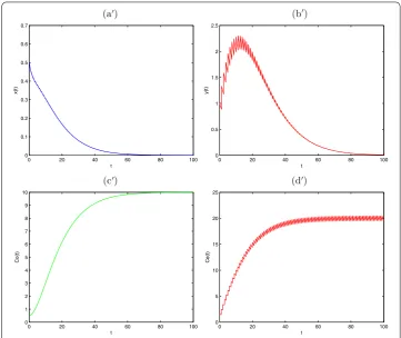
Figure 3 Globally asymptotically stable population-extinction periodic solution of system (2.1) with x(0) = 1,y(0) = 0.5,co(0) = 0.5,ce(0) = 0.5,a= 0.4,b= 1,d= 0.1,β= 0.05,μ= 1,f= 0.1,m= 0.1, g= 0.1,l= 0.25,D= 0.95,τ= 1. (a)Time-series ofx(t);(b)time-series ofy(t);(c)time-series ofco(t);
(d)time-series ofce(t).
stable population-extinction solution of system (.) is obtained, and the condition of the population permanence of system (.) is also obtained.
5.1 The simulation of system (2.1) affected by parameter
μ
If it is assumed thatx() = ,y() = .,co() = .,ce() = .,a= .,b= ,d= .,β= .,μ= ,f = .,m= .,g= .,l= .,D= .,τ= , then the population-extinction periodic solution of system (.) is globally asymptotically stable (see Figure ). If it is also assumed thatx() = ,y() = .,co() = .,ce() = .,a= .,b= ,d= .,β= .,
μ= ,f = .,m= .,g= .,l= .,D= .,τ= , then system (.) is permanent (see Figure ).
From the simulation experiments, the parameters μ obviously affect the dynamical behaviors of system (.). If all parameters of system (.) are fixed, when μ= , the population of system (.) will go extinct, whenμ= , system (.) is permanent. From Theorem ., we can easily deduce that there must exist a threshold μ∗. Ifμ>μ∗, the population-extinction periodic solution of system (.) is globally asymptotically stable. If
μ<μ∗, system (.) is permanent.
5.2 The simulation of system (2.1) affected by parameterD
If it is assumed that x() = ,y() = .,co() = .,ce() = .,a= .,b= , d= .,
population-Figure 4 The permanence of system (2.1) withx(0) = 1,y(0) = 0.5,co(0) = 0.5,ce(0) = 0.5,a= 0.4,b= 1, d= 0.1,β= 0.05,μ= 1,f= 0.1,m= 0.1,g= 0.1,l= 0.25,D= 0.1,τ= 1. (e)Time-series ofx(t);
(f)time-series ofy(t);(g)time-series ofco(t);(h)time-series ofce(t).
extinction periodic solution of system (.) is globally asymptotically stable (see Figure ). If it is also assumed thatx() = ,y() = .,co() = .,ce() = ., a= .,b= ,d= .,β= .,μ= ,f = .,m= .,g= .,l= .,D= .,τ = , then system (.) is permanent (see Figure ).
From the simulation experiments, the parametersDobviously affect the dynamical be-haviors of system (.). If all parameters of system (.) are fixed, whenD= ., the pop-ulation of system (.) will go extinct, whenD= ., system (.) is permanent. From Theorem ., we can easily deduce that there must exist a thresholdD∗. IfD>D∗, the population-extinction periodic solution of system (.) is globally asymptotically stable. If D<D∗, system (.) is permanent.
From the simulations of system (.), the diffusing parameterDof the population plays an important role in system (.). The environmental pollution will also reduce the bi-ological diversity of the nature world. Our results also provide a reliable tactic basis for practical biological resource management.
Competing interests
The authors declare that they have no competing interests.
Authors’ contributions
Author details
1School of Mathematics and Statistics, Guizhou Key Laboratory of Economic System Simulation, Guizhou University of
Finance and Economics, Guiyang, 550004, P.R. China.2School of Continuous Education, Guizhou University of Finance
and Economics, Guiyang, 550004, P.R. China.
Acknowledgements
Supported by National Natural Science Foundation of China (11361014, 10961008), the Science Technology Foundation of Guizhou Education Department (2008038), and the Science Technology Foundation of Guizhou (2010J2130).
Received: 10 February 2015 Accepted: 10 August 2015
References
1. Beretta, E, Solimano, F: Global stability and periodic orbits for two patch predator-prey diffusion delay models. Math. Biosci.85, 153-183 (1987)
2. Cui, JA, Chen, LS: Permanence and extinction in logistic and Lotka-Volterra system with diffusion. J. Math. Anal. Appl. 258(2), 512-535 (2001)
3. Freedman, HI: Single species migration in two habitats: persistence and extinction. Math. Model.8, 778-780 (1987) 4. Freedman, HI, Takeuchi, Y: Global stability and predator dynamics in a model of prey dispersal in a patchy
environment. Nonlinear Anal.13, 993-1002 (1989)
5. Freedman, HI, Takeuchi, Y: Predator survival versus extinction as a function of dispersal in a predator-prey model with patchy environment. Appl. Anal.31, 247-266 (1989)
6. Allen, LJS: Persistence and extinction in single-species reaction-diffusion models. Bull. Math. Biol.45(2), 209-227 (1983)
7. Beretta, E, Takeuchi, Y: Global stability of single species diffusion Volterra models with continuous time delays. Bull. Math. Biol.49, 431-448 (1987)
8. Jiao, JJ, Yang, XS, Cai, SH, Chen, LS: Dynamical analysis of a delayed predator-prey model with impulsive diffusion between two patches. Math. Comput. Simul.80, 522-532 (2009)
9. Hass, CN: Application of predator-prey models to disinfection. J. Water Pollut. Control Fed.53, 378-386 (1981) 10. Hsu, SB, Waltman, P: Competition in the chemostat when one competitor produces a toxin. Jpn. J. Ind. Appl. Math.
15, 471-490 (1998)
11. Jenson, AL, Marshall, JS: Application of surplus production model to access environmental impacts in exploited populations of Daphnia pulex in the laboratory. Environ. Pollut. A28, 273-280 (1982)
12. De Luna, JT, Hallam, TG: Effects of toxicants on population: a qualitative approach IV. Resource-consumer-toxicants model. Ecol. Model.35, 249-273 (1987)
13. Dubey, B: Modelling the effect of toxicant on forestry resources. Indian J. Pure Appl. Math.28, 1-12 (1997)
14. Freedman, HI, Shukla, JB: Models for the effect of toxicant in a single-species and predator-prey systems. J. Math. Biol. 30, 15-30 (1991)
15. Hallam, TG, Clark, CE, Jordan, GS: Effects of toxicant on population: a qualitative approach II. First order kinetics. J. Math. Biol.18, 25-37 (1983)
16. Zhang, BG: Population’s Ecological Mathematics Modeling. Publishing of Qingdao Marine University, Qingdao (1990) 17. Hallam, TG, Clark, CE, Lassider, RR: Effects of toxicant on population: a qualitative approach I. Equilibrium
environmental exposure. Ecol. Model.18, 291-340 (1983)
18. Liu, B, Chen, LS, Zhang, YJ: The effects of impulsive toxicant input on a population in a polluted environment. J. Biol. Syst.11, 265-287 (2003)
19. Liu, XN: Impulsive stabilization and applications to population growth models. J. Math.25(1), 381-395 (1995) 20. Lakshmikantham, V: Theory of Impulsive Differential Equations. World Scientific, Singapore (1989) 21. Liu, XN, Chen, LS: Complex dynamics of Holling type II Lotka-Volterra predator-prey system with impulsive
perturbations on the predator. Chaos Solitons Fractals16, 311-320 (2003)
22. Song, XY, Chen, LS: Uniform persistence and global attractivity for nonautonomous competitive systems with dispersion. J. Syst. Sci. Complex.15, 307-314 (2002)
23. Meng, XZ, Chen, LS: Permanence and global stability in an impulsive Lotka-VolterraN-species competitive system with both discrete delays and continuous delays. Int. J. Biomath.1(2), 179-196 (2008)
24. Jiao, JJ, et al.: An appropriate pest management SI model with biological and chemical control concern. Appl. Math. Comput.196, 285-293 (2008)
25. Murray, JD: Mathematical Biology, 2nd edn. Springer, Heidelberg (1993)
26. Takeuchi, Y: Global Dynamical Properties of Lotka-Volterra Systems. World Scientific, Singapore (1996)
27. Takeuchi, Y, Oshime, Y, Matsuda, H: Persistence and periodic orbits of a three-competitor model with refuges. Math. Biosci.108(1), 105-125 (1992)
28. Kuang, Y: Delay Differential Equation with Application in Population Dynamics, pp. 67-70. Academic Press, New York (1987)
29. Leung, AW: Optimal harvesting-coefficient control of stead-state prey-predator diffusive Volterra-Lotka system. Appl. Math. Optim.31, 219-241 (1995)
30. Alvarez, HR, Shepp, LA: Optimal harvesting of stochastically fluctuating populations. J. Math. Biol.37, 155-177 (1998) 31. Tang, SY, Chen, LS: The effect of seasonal harvesting on stage-structured population models. J. Math. Biol.48,
357-374 (2003)
32. Zhao, Z, Chen, LS: The effect of pulsed harvesting policy on the inshore-offshore fishery model with impulsive diffusion. Nonlinear Dyn.63, 521-535 (2011)