R E S E A R C H
Open Access
Research on modulation recognition with
ensemble learning
Tong Liu, Yanan Guan and Yun Lin
*Abstract
Modulation scheme recognition occupies a crucial position in the civil and military application. In this paper, we present boosting algorithm as an ensemble frame to achieve a higher accuracy than a single classifier. To evaluate the effect of boosting algorithm, eight common communication signals are yet to be identified. And five kinds of entropy are extracted as the training vector. And then, AdaBoost algorithm based on decision tree is utilized to confirm the idea of boosting algorithm. The results illustrate AdaBoost is always a superior classifier, while, as a weak estimator, decision tree is barely satisfactory. In addition, the performance of three diverse boosting members is compared by experiments. Gradient boosting has better behavior than AdaBoost, and xgboost creates optimal cost performance especially.
Keywords:Modulation scheme recognition, Ensemble learning, Boosting, Information entropy, Decision tree
1 Introduction
With the rapid progress of radio technology, it has influ-enced many fields such as communication reconnaissance and anti-reconnaissance. Communication modulation scheme is one of the most important technology in com-munication reconnaissance and anti-reconnaissance, and it has been widely used in military and civil fields [4–9]. Hence, the research of automatic modulation recognition (AMR) of digital signals should be pay more attention.
AMR is a central task to extract representative pa-rameters or features for defining the type of received unknown signals. In the past decade years, the approach for AMR can be mainly divided into two categories [4, 8–10]. The first one refers to the decision-theoretic method which utilizes the statistical computing on digital signals and then converts the AMR to the probability space by the threshold hypoth-esis to get the recognition results. However, it has obvious drawbacks requiring too many parameters of the signal and high algorithm complexity. The next approach mentions pattern recognition. It can be regarded as a mapping relationship, which means
mapping the time-series signals to feature fields, and the process of recognition just depends on the featured parameters. Compared with the former, pattern recog-nition occupies the advantage, an easy engineering im-plementation, and has a widespread application field. Generally, a large amount of data sets and training sets are employed to train the classifier, and then, a series of rather small sets, also called testing sets, try out the performance of the classifier. Above content has already displayed the primary steps for pattern recog-nition. However, there still exists a critical key issue of how to determine the classifier. A superior classifier can improve the overall recognition results, while a poor one will pull down the classification performance. A number of classifiers have been published, but the results are barely satisfactory under low signal to noise ratios (SNRs). To ameliorate the current state, we use the ensemble algorithm instead of single classifier. These algorithms, such as bagging and boosting, have been revealed more significant advantages than signal classifier [1–3, 33–37].
In this paper, the aim is to survey the performance of different boosting algorithms. From various algo-rithms, the AdaBoost, Gradient Boosting, and Extreme Gradient Boosting are selected. The ensemble algo-rithms can improve the recognition results by combin-ing a serious of base estimators (classifiers). Here, all * Correspondence:[email protected]
College of Information and Communication Engineering, Harbin Engineering University, Harbin, China
boosting methods are based on decision tree for the comparison of performance. The data set is composed of five different information entropies instead of con-ventional features.
The organization of this paper can be arranged as fol-lows. The next section is feature extraction. In this part, the feature is extracted for eight common digital signals, including 2ASK, 2FSK, BPSK, 4ASK, 4FSK, QPSK, 16QAM, and 64QAM. Power spectrum entropy, wavelet energy entropy, singular entropy, sample entropy, and Renyi entropy compose the input datasets. Section 3 provides the ensemble learning methodology. In Section 4, the experiments are shown and the details will be discussed later on. The summary is given in Section 5.
2 Feature extraction
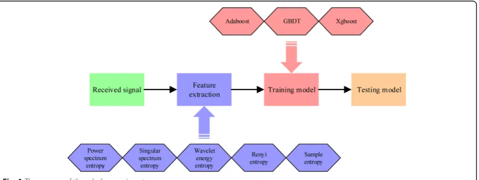
The processing of pattern recognition is shown in Fig. 1. We can roughly propose two key words for the whole processing: feature and classifier. No classifiers can work well with some invalid features. We have to choose the characteristics in a scientific way. This part analyzes the input data, i.e., features.
Different types of signal affect military and civilian application dissimilarly. And identifying the communi-cation signals precisely needs some powerful informa-tion. As a result, the powerful information is fertile such as amplitude, phase, frequency, high-order cumu-lants, and cyclic spectral features [11–17]. As time passes by, the feature extractor was not only focusing on the time-frequency analysis but entropy features [18–21, 38, 39]. The concept of entropy belongs to in-formation theory, which is a kind of measurement for the uncertainty of random events. It can be utilized to measure the uncertainty and complexity of the signal state distribution characteristic. The more entropy there is, the less stable the signal is. The capacity of carrying information can be distinguished by which is
the reason why entropy is suitable for applying in the AMR. In our work, the diverse five entropies are chosen to express the signal respectively. The detailed principles are displayed in the following part.
2.1 Power spectrum entropy
Power spectrum entropy reflects the complexity of the signal in the frequency domain and also the order de-gree with the signal energy. The frequency distribution will be obtained by Fourier transform. Relative to the time-sequence waveform, spectrum analysis embodies more internal characteristics. Here, the paper denotes the signal by {xi,i= 1, 2,…,N}, which will be converted
toX(ejw)after Fast Fourier Transform (FFT), and then, the power spectral density S(ejw) can be presented as the following expression:
S ejw ¼ 1 N
X
N−1
n¼0
xne−jw
2
ð1Þ
S(ejw) is the distribution of power in the frequency domain. If normalizing theS(ejw), then
pk¼ S e jw ð Þ
P∞
k¼1
S eð Þjw ð2Þ
H¼−X
∞
k¼1
pklog2pk ð3Þ
In (3), pk represents the kth ratio of the frequency to
whole spectrum and H is the power spectrum entropy. The less H is, the more concentrated it is in the main frequency point.
2.2 Singular spectrum entropy
Singular spectrum entropy [40] is a common entropy in the time domain. The extraction steps are grouped by
piecewise sequence, decomposition singular values, and
Assume the segment length is M, and xi can be
seg-mented by N−M. Then, the matrix A is given by (4). Signal’s information (δi) based onN−M basic vector is
got after decomposingA which is embodied in the way of the length of signal projection under the basic vector.
pi¼Pδi
The order degree of the signal information distribution is incarnated by singular spectrum entropy. If His rela-tively high, the signal order has a higher level.
2.3 Wavelet energy entropy
In the real world, most signals are non-stationary which leads to that the wavelet analysis is indispensable. Unlike FFT, wavelet transform is involved in two wavelet bases which can cover the frequency and time domains’ availability at the same time. Therefore, the local tiny features of signal can be described more finely.
Wf að ;bÞ ¼Df;φa;bE¼ 1ffiffiffiffiffiffi
The above equation is on behalf of wavelet transform on the signal f(t).The wavelet transform covers high-dimensional signals well, while the classical analytical method, FFT, is adopted to one-dimensional signals.
If the transformation scale is set to be j, then we use FFT on the wavelet signal:
Xð Þ ¼k X
. Similar to the above calcula-tion of these entropies, power spectrum and normalization for theX(k)can be denoted:
S kð Þ ¼ 1
According to the reference [22], the Renyi entropy is de-fined by:
When the input is two-dimensional probability density distribution f(x,y), then the Shannon entropy and α order Renyi entropy are denoted:
I pð Þ ¼−∬f xð ;yÞlog2f xð ;yÞdxdy
In this paper, a modified Renyi entropy, SPWVD Renyi entropy, is carried out. of smooth pseudo Wigner-Ville distribution (WVD) in the Cohen, because of the cross term in WVD.
2.5 Sample entropy
Sample entropy is a time series complexity measurement proposed by Richman [23, 24]. It can be considered as the modified approximate entropy. Now, sample entropy is defined as follows:
Here, the maximum distance between theith signalX(i) and the othersX(j) is calculated firstly,d[X(i),X(j)] = max {| X(i+k),X(j+k)|}. It must be noted that X(i) is composed imum is smaller than the setting threshold to all samples.
3 Classifiers
There is an algorithm originating from probably approxi-mately correct (PAC) learning model [25]. The concept of weak and strong learning is proposed by Valiant and Kearns. If the error rate is less than 0.5 slightly, which means the accuracy rate is just only better than random guessing, the algorithm can be considered as a weak learner [23, 24]. Then, another issue to ponder is how to boost the weak learners to be strong learners. A polynomial-time boosting method is come up by Schapire in 1989 [26], which is the prototype of boosting algorithm. In recent years, the appli-cation of boosting algorithm has become popular among various classifiers. As a machine learning method, ensemble boosting devotes to finding rough rules of thumb other than getting a high prediction rate rule. Especially, its superiority is reflected in avoiding overfitting and high probability of classification in high-dimensional space. In this paper, we employ boosting classifier instead of single classifier to build a high accuracy for the pattern recognition.
3.1 AdaBoost
Boosting is a cluster of algorithms. In 1995, a converted boosting, adaptive boosting (AdaBoost), was introduced by Freund and Schapire [27]. AdaBoost algorithm is one of the most famous representatives; therefore, it aims at trans-forming weak learners to strong ones. One of the cushy comprehensions is linear combination based on these weak learners or estimators for the AdaBoost.
Here takes a binary classification as an example to explain the process:
In the above process,wijdenotes the weight for thej
th
sample in theithround.
D is just sample weight set. AdaBoost combines a series of estimators by line, andαmis another weight or a
coefficient for the estimator. From the equality relation-ship, it is obvious thatαmis inversely proportional toem.
AndZmrepresents the normalization ofwijwhich is
satis-fied with the probability. In addition, we will find wij
-depends on the last round result to upgrade where the adaptive comes from. All weak learners are not alone with each other but link closely.
The performance of ensemble method is closely related to weak learners. In the real situation, AdaBoost with decision tree is the best off-the-shelf classifier [28]. As a result, the whole simulation is based on the only weak classifier, i.e., decision tree.
3.2 Gradient boosting
Another stagewise boosting member is gradient boosting (GB) derived by Friedman [29, 30]. The principle idea of gradient boosting is to construct the new model based on the negative gradient of the previous loss function which is related to the former iteration rounds. In the machine learning, loss function is the key issue to solve, which em-bodies the relationship between prediction and target. The less the loss function is, the higher the precision is. If the loss function declines consecutively with the iteration process, a conclusion that the model changes sequentially along a superior direction can be inferred. Gradient of loss function is the superior direction.
Considering the supervised classification, there is an ex-pected objective to find an approximation ruleFbð ÞÞx to fit theF(x). Here, the definition of loss function isL(y,F(x)):
Fb¼ arg min F
L yð;FÞ ð
16Þ
where F denotes the linear combination of some weak learners (Gi(x)) with weights (γi). AndF tries minimizing
the value of loss function on the input vector. So, the algorithm initializes a constant functionF0(x),
F0ð Þ ¼x arg min
γ
Xn
i¼1
L yði;γÞ ð17Þ
Similar with AdaBoost, if the decision tree is selected as the estimator, the algorithm will be the gradient boosting decision tree (GBDT), a shining classifier, which can be applied in many fields.
At the beginning of this section, we have mentioned there are a lot of member algorithms in the boosting method family. Gradient boosting and AdaBoost are two common ones of them. If we view from an abstract point, both of them get solved with the help of convex loss function. But gradient boosting can get more types of loss function. What is more, GB could deal with both regression and classification. In classification mode, log loss function is always the best objective function while AdaBoost will choose exponential loss. If you want to tell them from the fundamental element, the crucial question is how to identify the model. AdaBoost utilizes the mis-classification to adjust the weight of weak learners whereas GB applies Negative gradient to ameliorate.
3.3 Extreme gradient boosting
During the last years, data mining and data analysis become the current topic with the rise of alpha go. Our life is full of these words such as big data and arti-ficial intelligence. Boosting family also has a vicissitude with time. A novel boosting method occurs in the Kaggle, extreme gradient boosting, simply xgboost.
Xgboost, an implementation of GBDT, offers a novel tree searching: end to end [31, 32]. The algorithm has advantages in distributed computing, solving the sparse, and avoiding overfitting better. In other words, the amount of calculation reduces greatly and the split direction is learned automatically. For overfitting, regular terms are appended to the objective.
Different from conventional GBDT, xgboost performs second-order Taylor expansion on the loss function replacing the first derivative. Based on GBDT, xgboost can be described as the following:
L¼X
i
l yð ;FÞ þX k
Ωð ÞGk ð18Þ
Here, we use l as the training loss function as above, and Lis the real loss function for xgboost method. The other notations are consistent with the ones in other mentioned boosting methods. G is the weak estimator (decision tree) and F represents prediction. Moreover, the complexity of the decision trees (Ω(Gm)) is added
into the loss to construct the objective function. The definition of regular term,Ω(Gm), is showed as:
Ωð Þ ¼G γT þ1
2λ
XT j¼1wj
2 ð19Þ
whereTis the number of leaves of the decision tree and wj2 means L2 norm of leaf scores. γ is the threshold to
control the split of nodes, andλis just on behalf of coef-ficient to preserve overfitting which is a unique charac-teristic. More details are demonstrated in reference [31]. Then, the equation can be transformed as:
Lm¼X
From the equation, the other main variables can be de-noted respectively: gi¼∂Fm−1l yi;Fm−1
, the first and second derivative on loss function.
4 Experiments
After introduction of methodology, AMR experiment to evaluate ensemble methods is proposed in this part. We consider the eight types of modulation schemes including 2ASF, 2FSK, BPSK, 4ASK, 4FSK, QPSK, 16QAM, and 64QAM. For every signal, sampling rate is 16 KHz and carrier frequency is 4 KHz. The other parameters are listed here such as number of symbols (125), symbol rate (1000), and length of signal (2000). The range of SNR is between−10 and 20 dB with the 3 dB step length.
Data set is divided into training data and testing data. The first one covers 8000 samples in every SNR while the other one has 4000 samples. Every modulation scheme extracts 1500 samples for one SNR.
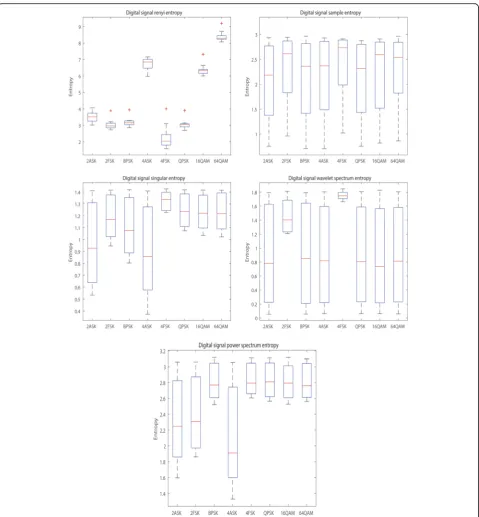
The experiment begins with the extraction entropy feature. From Fig. 2, the distribution of feature where entropy acts the communication scheme on the 11 SNRs is shown. Because these entropies are discrete points, boxplot that embodies the distribution of discrete data well has been used to analyze characteristics. The reason why the range of maximum and minimum is immense is that the boxplot is made under all SNRs. Median layout is well-proportioned that maybe contribute to the classi-fication. One of the five pictures looks contrary from the others. The Renyi entropy boxplot displays some points labeled by “+”, called extreme outliers, which causes some inference to recognition result. In addition, data is more concentrated, which means the feature is not sen-sitive to noise. Wavelet spectrum entropy affects the all modulation similarly except the type of FSK. As a feature, its contribution may be less than others. Furthermore, QPSK, 16QAM, and 64QAM almost are similar with each other except Renyi entropy. This mostly results in some misclassification.
4.1 AdaBoost with weak learners
single with groups. Decision tree (DT) is the only candi-date. The result is shown in the graph.
Shown in Fig. 3, with the depth of tree higher, the recog-nition rate of DT becomes better. For example, when the SNR is−10 dB, two-tier DT is just a random guessing be-cause the recognition probability is about 50%, whereas DT based on four layers can acquire precision more than
70%. DT is a tree structure from one node split binary branches according to some special conditions which point to GINI information Branch connects two nodes: one is the generation, parent node; the other is child node. Child follows the parent to spill continuously until it meets the decision rules. Consequently, it is a capability to embody classifying by setting a higher depth of tree. The
lusher the tree evolves, the more complex the algorithm is and as a result the higher the accuracy is.
However, there is a worrying phenomenon in the above picture. When the SNR reaches 5 dB, DT’s ability goes down drastically. We have no choice but to con-sider whether the cause is from features or base classi-fiers. The following picture will interpret the reason.
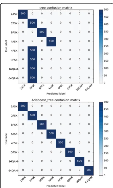
The confusion matrix is used to exhibit details of classification. The column denotes the real target while the row denotes the predicted label. It is a visualization tool to compare the classification results and actual measured value primarily.
The left matrix is the result of accuracy of decision tree based on 4 layers. For each signal, there are 500 samples to test the model. Modified model can identify the digital signals adequately except QPSK, 16QAM, and 64QAM. Model feels confused with regard to QPSK, QAM, and 2FSK. It allots wrong label, i.e., 2FSK, to them. Moreover, none of them can be escaped which means the five entropy features does not work anymore. These features no longer have their unique characteristics.
The right confusion matrix shows the AdaBoost rec-ognition rate. Although the base learner has a low grade, ensemble has an opposite one. This is the en-semble’s original idea which comes from PAC and re-quires just about 50% probability. In Fig. 4, two confusion matrixes verify the conclusion that boosting has the ability to enhance the accuracy of weak learners once again. As for the features, although they demonstrate a little anti-common sense which is work-ing badly under high SNR, this is not a key issue with the performance comparison text and offers an evidence to support the ensemble theory. So it will not be discussed much anymore.
Fig. 3Comparison of different tree depth between decision tree and AdaBoost algorithm with 800 rounds iteration. The right column always denotes decision tree with diverse depth, and the left one is AdaBoost. The correct order in legend is from left to right and up to down
4.2 Comparison of boosting
The conclusion that AdaBoost algorithm converts base learner into a strong one successfully can be made. As the same with other algorithms, boosting algorithm also is a family method. Assorted deformation algorithms have been proposed by the amount of researchers and studies during the past decades. Two epidemical arithmetic based on tree structure stand out from these boosting members. The next experiment will show the comparison between the popular and classical arithmetic.
Seen from Table 1, every column includes a series of classification rate by means of three individual boosting al-gorithms. The recognition probability of eight typed signal is satisfied in all SNRs. All of the results based on three depth of tree are done with 100 rounds except xgboost that only iterates 20 times. The trend of recognition prob-ability emerges upward from vertical direction. If we re-gard from horizontal perspective, the effect of GBDT is proximal to xgboost. Notwithstanding boosting achieve a higher outcome, gradient boosting seems better than others. In the case of −10 dB SNR, AdaBoost algorithm gets probability 78% but gradient boosting’s average is probability 85%. Although these two gradient boosting al-gorithms are approximate, the xgbooost occupies less it-erative times; that is to say, it masters high proceeding speed but less resources consumption. Modulation scheme recognition is an engineering project in civil and
military application. Therefore, performance of xgboost al-gorithm is excellent.
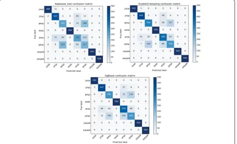
As the same as former, confusion matrix is utilized to show the classification details. We want to analyze the probability of classification for every sigma.
In Fig. 5, confusion matrixes give the proportion that every signal recognition result. The confusion matrix presents visualization of the performance of three
Table 1Probability of different ensemble learning
SNR Classifier
AdaBoost GBDT Xgboost
−10 dB 0.783 0.8501 0.8465
−7 dB 0.894 0.928 0.928
−4 dB 0.993 0.993 0.993
−3 dB 1.000 1.000 1.000
−1 dB 1.000 1.000 1.000
2 dB 1.000 1.000 1.000
5 dB 1.000 1.000 1.000
8 dB 1.000 1.000 1.000
11 dB 1.000 1.000 1.000
14 dB 1.000 1.000 1.000
17 dB 1.000 1.000 1.000
20 dB 1.000 1.000 1.000
contrast algorithms which brings more details than ac-curacy. Although some signal is misclassified, the recog-nition result is satisfied from the three confusion matrixes. The type of ASK and QAM can be identified correctly, while the others are mixed together. For BPSK, almost half of the samples are labeled with QPSK. Meanwhile, QPSK is acknowledged as BPSK. Most of the wrong 4FSK is predicted as QPSK, some as BPSK and the rest is considered as 2FSK. In general, PSK can-not be distinguished greatly. However, the excellent boosting members reduce the number of wrong samples. Xgboost is the derivative of GBDT; therefore, the result is similar but better than AdaBoost. Even so, no matter which ensemble learning is chosen, the law of identifica-tion will not be influenced unless the SNR alters.
5 Conclusions
In order to enhance the probability of communication digital signal recognition, in this paper, we bring in ensem-ble learning based on boosting algorithm. All of three boosting member algorithms can obtain a higher accuracy than weak classifier. First, five different information en-tropy of communication signals are extracted as the input training data set of classifiers. A boxplot is used to show the distribution of discrete features, and a similarity for QPSK, 16QAM, and 64QAM is also displayed. And then the experiment starts from the comparison between the AdaBoost algorithm and decision tree algorithm with un-certain depth of tree. The result exhibits that AdaBoost can improve the performance of decision tree despite the entropy feature work badly when SNR is over 2 dB. At last, another check experiment is made to confirm proper-ties of each boosting member. It is obviously seen from the table of recognition result that gradient boosting is su-perior to classical AdaBoost a little. And the state-of-art boosting algorithm, named xgboost, may be more suitable for modulation scheme classification without less iteration times and higher precision.
Acknowledgements
This work is supported by the National Nature Science Foundation of China (61301095), the Key Development Program of Basic Research of China (JCKY2013604B001), and the Fundamental Research Funds for the Central Universities (GK2080260148 and HEUCF1508). We gratefully thank very useful discussions of reviewers.
Funding
The research is funded by the International Exchange Program of Harbin Engineering University for Innovation-oriented Talents Cultivation.
Authors’contributions
The authors have contributed jointly to all parts of the preparation of this manuscript, and all authors read and approved the final manuscript.
Competing interests
The authors declare that they have no competing interests.
Publisher’s Note
Springer Nature remains neutral with regard to jurisdictional claims in published maps and institutional affiliations.
Received: 21 July 2017 Accepted: 8 September 2017
References
1. E Bauer, R Kohavi. An empirical comparison of voting classification algorithms: bagging, boosting, and variants. Mach. Learn.36(1), 105–139 (1999)
2. J Bergstra, N Casagrande, D Erhan, et al. Aggregate features and AdaBoost for music classification. Mach. Learn.65(2–3), 473–484 (2006)
3. P Viola, M Jones.Fast and Robust Classification Using Asymmetric AdaBoost and a Detector Cascade. Advances in Neural Information Processing Systems
(2002), pp. 1311–1318
4. A Hossen, F Al-Wadahi, JA Jervase. Classification of modulation signals using statistical signal characterization and artificial neural networks. Eng. Appl. Artif. Intell.20(4), 463–472 (2007)
5. E Azzouz, AK Nandi. Automatic Modulation Recognition of Communication Signals. J Franklin. Instit.46(4), 431-436 (1998)
6. D Grimaldi, S Rapuano, L De Vito. An automatic digital modulation classifier for measurement on telecommunication networks. IEEE Trans. Instrum. Meas.56(5), 1711–1720 (2007)
7. OA Dobre, A Abdi, Y Bar-Ness, et al. Survey of automatic modulation classification techniques: classical approaches and new trends. IET Commun. 1(2), 137–156 (2007)
8. JL Xu, W Su, M Zhou, Likelihood-ratio approaches to automatic modulation classification. IEEE Trans. Syst. Man Cybern. Part C Appl. Rev.41(4), 455–469 (2011)
9. A Swami, BM Sadler. Hierarchical digital modulation classification using cumulants. IEEE Trans. Commun.48(3), 416–429 (2000)
10. Z Tian, Y Tafesse, BM Sadler. Cyclic feature detection with sub-Nyquist sampling for wideband spectrum sensing. IEEE. J. Top. Signal. Process.6(1), 58–69 (2012)
11. OA Dobre, Y Bar-Ness, W Su. Higher-order cyclic cumulants for high order modulation classification. Military Communications Conference, 2003. MILCOM'03. 2003 IEEE. IEEE.1, 112–117 (2003)
12. CM Spooner. Classification of co-channel communication signals using cyclic cumulants Signals, Systems and Computers, 1995. 1995 Conference Record of the Twenty-Ninth Asilomar Conference on IEEE.1, 531-536 (1995) 13. E Like, VD Chakravarthy, P Ratazzi, et al. Signal classification in fading
channels using cyclic spectral analysis. EURASIP J. Wirel. Commun. Netw. 2009(1), 879812 (2009)
14. A Polydoros, K Kim. On the detection and classification of quadrature digital modulations in broad-band noise. IEEE Trans. Commun.38(8), 1199–1211 (1990)
15. LV Dominguez, JMP Borrallo, JP Garcia, et al. A general approach to the automatic classification of radiocommunication signals. Signal Process. 22(3), 239–250 (1991)
16. OA Dobre, M Oner, S Rajan, et al. Cyclostationarity-based robust algorithms for QAM signal identification. IEEE Commun. Lett.16(1), 12–15 (2012) 17. WA Gardner. The spectral correlation theory of cyclostationary time-series.
Signal Process.11(1), 13–36 (1986)
18. SU Pawar, JF Doherty. Modulation recognition in continuous phase modulation using approximate entropy. IEEE. Trans. Inf. Forensics. Secur. 6(3), 843–852 (2011)
19. SM Pincus. Approximate entropy as a measure of system complexity. Proc. Natl. Acad. Sci.88(6), 2297–2301 (1991)
20. H. Kantz, T. Schreiber,Nonlinear time series analysis. Technometrics43(4):491 (1999)
21. S Kadambe, Q Jiang. Classification of modulation of signals of interest. Digital Signal Processing Workshop, 2004 and the 3rd IEEE Signal Processing Education Workshop. 2004 IEEE 11th. IEEE, 226–230 (2004)
22. RG Baraniuk, P Flandrin, AJEM Janssen, et al. Measuring time-frequency information content using the Rényi entropies. IEEE Trans. Inf. Theory47(4), 1391–1409 (2001)
24. M Kearns, L Valiant. Cryptographic limitations on learning Boolean formulae and finite automata. JACM41(1), 67–95 (1994)
25. LG Valiant. A theory of the learnable. Commun. ACM27(11), 1134–1142 (1984)
26. RE Schapire. The strength of weak learnability. Mach. Learn.5(2), 197–227 (1990)
27. Y Freund, RE Schapire,A Desicion-Theoretic Generalization of On-line Learning and an Application to Boosting. European Conference on Computational Learning Theory(Springer, Berlin, Heidelberg, 1995), pp. 23–37 28. L Breiman. Bagging predictors. Mach. Learn.24(2), 123–140 (1996) 29. JH Friedman, Greedy function approximation: a gradient boosting machine.
Ann. Stat., 1189–1232 (2001)
30. JH Friedman. Stochastic gradient boosting. Comput. Stat. Data. Anal.38(4), 367–378 (2002)
31. T Chen, C Guestrin.XGBoost: A Scalable Tree Boosting System(ACM SIGKDD International Conference on Knowledge Discovery and Data Mining ACM, 2016), pp. 785-794
32. L Torlay, M Perrone-Bertolotti, E Thomas, et al. Machine learning–XGBoost analysis of language networks to classify patients with epilepsy. Brain. Informatics.11, 1–11 (2017)
33. Y Freund, RE Schapire, Experiments with a new boosting algorithm. Icml96, 148–156 (1996)
34. Y Freund, R Iyer, RE Schapire, et al. An efficient boosting algorithm for combining preferences. J. Mach. Learn. Res.4, 933–969 (2003)
35. H Drucker, R Schapire, P Simard.Improving Performance in Neural Networks Using a Boosting Algorithm, Advances in neural information processing systems (1993), pp. 42–49
36. NC Oza. Online bagging and boosting Systems, man and cybernetics, 2005 IEEE international conference on IEEE.3, 2340-2345 (2005)
37. MC Tu, D Shin, D Shin. Effective diagnosis of heart disease through bagging approach. Biomedical Engineering and Informatics, 2009. BMEI'09. 2nd International Conference on IEEE. 1-4 (2009)
38. J Li, Y Li, Y Lin. The application of entropy analysis in radiation source feature extraction. J Projectiles Rockets Missiles Guid31(5), 155–160 (2011) 39. ZY He, YM Cai, QQ Qian. A study of wavelet entropy theoryand its
application in electric power system fault detection. Proc CSEE5, 006 (2005) 40. J Li, Y Ying. Radar signal recognition algorithm based on entropy theory.