A B spline finite element method for nonlinear differential equations describing crystal surface growth with variable coefficient

R E S E A R C H

Open Access

A B-spline finite element method for

nonlinear differential equations describing

crystal surface growth with variable

coefficient

Dandan Qin

_{, Yanwei Du}

_{, Bo Liu}

_{and Wenzhu Huang}

*_{Correspondence:}

[email protected] 1_{College of Mathematics, Jilin} University, Changchun, P.R. China 2_{Fundamental Department,} Aviation University of Air Force, Changchun, P.R. China Full list of author information is available at the end of the article

Abstract

In this paper, an efficient finite element scheme is presented for a class of fourth-order nonlinear parabolic problems with variable coefficient. To deal with second-order term in weak formulation, we choose the cubic B-spline function as a trial function. Rigorous error estimates are derived for both semi-discrete and fully-discrete schemes. We provide a numerical example to confirm our theoretical results.

Keywords: Cubic B-spline; Finite element method; Nonlinear parabolic equation; Variable coefficient; Error estimate

1 Introduction

Molecular beam epitaxy (MBE) is a widely practiced technique for depositing atoms from a vapor phase onto a surface. The technique is very important in growing thin films [1,2]. Crystal surface growth has recently received increasing interest in materials science [3,4]. A reason is that it could be used in the design of semi-conductors.

In the analysis of MBE,H(x,t) is the hight of the surface above the substrate plane, and

H(x,t) satisfies the current continuity equation

Ht+∇ ·Jsurface{H}=F, (1)

whereFis the incident mass flux out of the molecular beam.Jsurface, which depends on the

whole surface configuration, is the systematic current. Keeping only the most important terms in a gradient expansion, subtracting the mean heightH=Fu, and using appropri-ately rescaled units of height, distance, and time [5], one can get

ut= –γ 2u–μ∇ ·f∇u2∇u, (2)

whereγ andμare two positive constants. In equation (2), the linear term models relax-ation through adatom diffusion driven by the surface free energy [6], while the nonlinear term simulates the nonequilibrium current [7]. A Burton–Cabrera–Frank type theory [8,

9] indicates the formulaf(s2_{) =} 1

1+s2 [5]. Hence, we attain the following form:

ut+γ 2u+μ∇ ·

_∇

u

1 +|∇u|2

= 0, (x,t)∈Ω×(0,T), (3)

whereΩ⊂R2is a bounded domain with smooth boundary.

In [10], Grasselli et al. showed that equation (3) endowed with no-flux boundary con-ditions generates a dissipative dynamical system under very general assumptions on∂Ω

on a phase-space ofL2_{type. In the limit of weak desorption, Pierre-Louis et al. derived a}

1D case of equation (3) for vicinal surface growing in the step flow mode [11]. This limit turned out to be singular, and nonlinearities of arbitrary order need to be taken into ac-count. For 1D case of equation (3), Zhao et al. proved that the Hermite finite element method has the convergence rate ofO(t+h3) (see [12]).

The finite element method (FEM) [13–18], as a type of an important numerical tool for solving differential equations, has a long history. For 1D Cahn–Hilliard equation, Zhang derived the error estimates of FEM [19]. Elliott and French [20] studied a continuous in-time finite-element Galerkin approximation for two-dimensional Cahn–Hilliard equa-tion. In [21], Barrett et al. discussed the FEM for a fourth-order nonlinear degenerate parabolic equation. An iterative scheme, which solves the resulting nonlinear discrete sys-tem, is analyzed. In [22], Kästner et al. considered a numerical convergence study of the Cahn–Hilliard phase-field model within an isogeometric finite element analysis frame-work.

We also want to introduce the development history of the B-spline method. In 1946, the B-spline method was first presented in Schoenberg’s paper [23]. Curry and Schoenberg in-troduced one element B-spline functions in 1966 (see [24]). In 1976, de Boor extended B-spline to multiple situations [25]. Box-splines [26], simple splines [27], and conical splines [28], which were presented by de Boor, Micchelli, and Dahmen respectively, are the ele-gant forms of different functional forms of the multivariate B-splines. B-splines have been widely used in various fields of numerical analysis [29–31]. Hall studied the cubic B-spline interpolation [32,33]. There are several papers which study the B-spline FEM [34–39].

B-splines have better smoothness than the Hermite type elements, for example, quadrat-ic B-splines are inC1_{(–∞, +∞). Unfortunately, the convergence order of the FEM using}

quadratic B-splines is lower. Besides, Hermite type elements have two types of different basis functions, but the B-spline finite element only has one type of basis functions. So we consider the cubic B-spline FEM for a fourth-order nonlinear parabolic equation with variable coefficient. The convergence order of the B-spline FEM is equal to that of the Hermite FEM in paper [12].

The outline of this paper is as follows. In the next section, some basic definitions and results are introduced. In Sect.3, we study the semi-discrete approximation and derive its convergence rate. In Sect.4, the error estimate of the fully-discrete scheme is discussed. In Sect.5, some numerical experiments are presented to confirm our theoretical results.

Throughout this paper, the lettersCandCdenote generic constants independent of the division size not necessarily the same at different occurrences. On the other hand, we denoteL2_,L∞_,Hk_{norms inIby · ,| · |}

2 Preliminaries

For a 1D case of equation (3), considering the fourth-order term with the variable co-efficient and the suitable initial and boundary value conditions, we obtain the following problem:

⎧ ⎪ ⎪ ⎨ ⎪ ⎪ ⎩

ut+ (α(x,t)uxx)xx+μ(_1+|u_ux_x|2)x= 0, (x,t)∈I×(0,T), u(x,t) =ux(x,t) = 0, (x,t)∈∂I×(0,T),

u(x, 0) =u0(x), x∈I,

(4)

whereI= [0, 1]. The variable coefficientα(x,t) satisfies the assumption

α(x,t),∂α

∂t(x,t)∈C

I×[0,T], (5)

and there exist three positive constantss,S, andMsuch that 0 <s≤α(x,t)≤S< +∞, (x,t)∈I×[0,T],

∂α

∂t

≤M, (x,t)∈I×[0,T].

(6)

Remark2.1 Notice that the essential boundary conditions areu(0,t) =u(1,t) =ux(0,t) =

ux(1,t) = 0. Then we define the following space:

H₀2(I) =w;w∈H2(I),w(0,t) =w(1,t) =wx(0,t) =wx(1,t) = 0

.

Letkbe any positive integer andϕk(x) denote thekth-order B-spline with knots at the

setZof integers such thatsupp(ϕk) = [0,k]. More precisely,ϕk(x) is defined recursively by

Nk(x) = (Nk–1∗N1)(x) = 1

0

Nk–1(x–t)dt

with

N1(x) =χ[0,1]= ⎧ ⎨ ⎩

1, x∈[0, 1], 0, else.

N4(x) is obviously the cubic B-spline and can be expressed as

N4(x) = ⎧ ⎪ ⎪ ⎪ ⎪ ⎪ ⎪ ⎪ ⎪ ⎨ ⎪ ⎪ ⎪ ⎪ ⎪ ⎪ ⎪ ⎪ ⎩ 1

6x3, x∈[0, 1],

–1₂x3_{+ 2x}2_{– 2x+}2

3, x∈[1, 2], 1

2x

3_{– 4x}2_{+ 10x–}22

3, x∈[2, 3],

–1₆(x– 4)3_{, x∈[3, 4],}

0, else.

(7)

The variational problem related to (4) is: Findu=u(·,t)∈H2

0(I) (0≤t≤T) such that ⎧

⎨ ⎩

(ut,v) + (α(x,t)D2u,D2v) =μ(₁₊Du_|Du|2,Dv), ∀v∈H02(I),

u(x, 0) =u0(x), x∈I,

(8)

whereDu=∂_∂u_x. We give the existence of the solution of problem (8) in the following the-orem (see [12]).

Theorem 2.1 Suppose that u0∈H02(I).Then there exists a unique global solution u(x,t)

for problem(8)such that

u∈L∞0,T;H₀2(I)∩L20,T;H4(I), ut∈L20,T;L2(I).

3 Semi-discrete scheme

The interval 0 =x0<x1<· · ·<xL= 1 is divided intoLequal finite elements byh= 1/L.

Considering that the approximate solution must satisfy the boundary conditions, we in-troduce extended virtual nodesx–3,x–2,x–1,xL+1,xL+2,xL+3. Ifϕi(x) =N4(x–_hxi), thusϕi(x)

are the cubic B-spline functions with knots at the pointsxi. Actually, B-spline basis functions are constructed as follows:

ϕ–3(x),ϕ–2(x),ϕ–1(x),ϕ0(x), . . . ,ϕL–4(x),ϕL–3(x),ϕL–2(x),ϕL–1(x)

, where

ϕ–3(x) = 6ϕ–3(x),

ϕ–2(x) =ϕ–2(x) – 4ϕ–3(x),

ϕ–1(x) =ϕ–1(x) –

1

2ϕ–2(x) +ϕ–3(x),

ϕL–3(x) =ϕL–3(x) –

1

2ϕL–2(x) +ϕL–1(x),

ϕL–2(x) =ϕL–2(x) – 4ϕL–1(x),

ϕL–1(x) = 6ϕL–1(x).

For convenience, we still denote the basis functions as{ϕi(x)}. The basis functions satisfy

the following properties:

ϕ–3(0) = 1, ϕi(0) = 0 (i= –3), ϕi(0) = 0 (i= –3, –2), ϕL–1(1) = 1, ϕi(1) = 0 (i=L– 1), ϕi(1) = 0 (i=L– 1,L– 2).

The B-spline parametrization is generally defined in the domain [0, 1]. In this paper, we useN4(x) to define the shape functions, which is convenient in computing integrals.

Let Uh be the cubic B-spline space, thus Uh ⊂H2

0(I). The approximation solution

uh(x,t)∈Uhsatisfies

uh(x,t) = L–3

i=–1

δi(t)ϕi(x),

The semi-discrete finite element scheme based on B-splines for problem (8) is: Find

uh=uh(·,t)∈Uh(0 <t≤T) such that

⎧ ⎨ ⎩

(uh,t,vh) + (α(x,t)D2uh,D2vh) =μ(₁₊Du_|Duh

h|2,Dvh), ∀vh∈Uh,

(uh(0) –u0,vh) = 0, ∀vh∈Uh.

(9)

In order to deduce the error estimates of the B-spline FEM, we introduce the following lemma.

Lemma 3.1 The elliptic projection Rh:u→Rhu∈Uhis defined by

a(u–Rhu,vh)≡

α(x,t)D2(u–Rhu),D2vh

= 0, ∀vh∈Uh. (10)

It then follows from(6)and(10)that

a(u,u) =aα(x,t)u,u≥Cu2₂, ∀u∈H₀2(I), (11)

where C is a positive constant depending onα(x,t).Hence,a(u,v)is a symmetrical positive definite bilinear form,and(see[13])

u–Rhu+hu–Rhu1+h2u–Rhu2≤Ch4u4. (12)

Firstly, we analyze the boundedness of the semi-discrete scheme.

Theorem 3.1 For uh(0)∈H02(I),there exists a unique solution uh(t)∈Uhfor problem(8)

such that

uh(t)₂≤Cuh(0)₂, 0≤t≤T, (13)

where C is a positive constant depending onα(x,t),μ,and T,but independent of mesh size h.

Proof According to ordinary differential equation theory, there exists a unique local solu-tion to problem (9) in the interval [0,tn). If we have (13), then according to the extension theorem, we can obtain the existence of unique global solution. So, we only need to prove (13).

Settingvh=uhin (9) and based on (6), we get 1

2

d dtuh

2_+sD2_uh2_≤

μ

Duh

1 +|Duh|2

,Duh

≤μDuh2

= –μD2uh,uh≤ s

2D

2_uh2₊μ2

2suh

2_.

Therefore

d dtuh

2_+sD2_uh2_≤μ2

s uh

Then

Integrating (15) with respect tot, we have

uh(t)

A direct calculation gives

Byε-inequality, we have

μ

Integrating (18) with respect tot, we obtain

D2uh(t)2≤e16M+25μ

Theorem 3.2 Let u be the solution to(8),uh be the solution to(9).Assume that u(0)∈

Using (6) andε-inequality, we can deduce that

Hence

By Gronwall’s inequality, we get

θ2≤Cθ(0)2+

Next, we deal with theH2_-estimate.

Theorem 3.3 Let u be the solution to(8),uh be the solution to(9).Assume that u(0)∈

H4_(I),u,u

t∈L2(0,T;H4(I)),and the initial value satisfies

u(0) –uh(0)₂≤Ch2u(0)₄. (31)

Then we have the following error estimate:

where

To derive the theorem, we give the following estimate:

Integrating (36) with respect tot, we have

D2θ2≤CD2θ(0)2+

4 Fully-discrete scheme

The fully-discrete finite element scheme for problem (8) is: Findun

h∈Uh(n= 1, 2, . . . ,N)

such that

⎧ ⎨ ⎩

(∂tunh,vh) + (α(x,tn,θ)D2u n,θ

h ,D2vh) =μ( Dun_h,θ

1+|Dun_h,ϑ|2,Dvh), ∀vh∈Uh,

(u(0),vh) = (u0

h,vh), ∀vh∈Uh,

(39)

whereNis a given positive integer,t=T/Ndenotes the time step size,tn=ntand

∂tun_h=un_h–un_h–1/t,

tn,θ=θtn+ (1 –θ)tn–1,

un_h,θ=θu_hn+ (1 –θ)un_h–1,

un_h,ϑ=ϑu_hn+ (1 –ϑ)un_h–1.

Whenθ=ϑ= 1 andθ=ϑ=1

2, the schemes are the backward Euler and Crank–Nicolson

finite element scheme, respectively.

In this paper, we chooseθ= 1,ϑ= 0. The fully-discrete finite element scheme is

⎧ ⎨ ⎩

(∂tunh,vh) + (α(x,tn)D2unh,D2vh) =μ( Dun_h

1+|Dun_h–1|2,Dvh), ∀vh∈Uh,

(u(0) –u0

h,vh) = 0, ∀vh∈Uh.

(40)

From the above formulation, ifun–1

h is known, the fully-discrete finite element scheme is

linear. We give the next estimate.

Theorem 4.1 Let un_{be the solution to problem(8),u}n

hbe the solution to the fully-discrete scheme(40).Assume that u(0)∈H4_(I),ut∈L2_(0,T;H4_(I)),utt∈L2_(0,T;L2_{(I)),and u}

0h∈ Uhsatisfies

u(0) –u0_h≤Ch4u(0)₄. (41)

For sufficiently smallt,there exists a constant C independent of h,t,and n such that

un–un_h≤Ct+h3. (42)

Proof Letρn_=un_–Rhun_andθn_=Rhun_–un

h. Thenun–unh=ρn+θn, and

∂tθn,vh

+αnD2θn,D2vh

=rn,vh+μ

Dun

1 +|Dun|2–

Dun h

1 +|Dun–1

h |2

,Dvh

, (43)

where

∂tθn=

Takingvh=θn_{in (43), using Lemma3.1andε-inequality, we get}

We can easily obtain

Dθn2= –θn,D2θn≤ 1

In addition, we have

≤C

One can easily get

Thus

θn2≤Ct n–1

i=1

θi2+C(t)2+h6. (52)

Using the discrete Gronwall inequality and Lemma3.1, we get the error estimate (42). Although we assume thatα(x,t) is a smooth function in (5),α(x,t)∈W1,∞_(0,T;W1,∞_(I))

is enough.

It is difficult to estimate the nonlinear term which affects the convergence order of the schemes. It leads to the failure of the optimal convergence.

5 Numerical approximation

In this section, we consider the following equation:

⎧ ⎪ ⎪ ⎨ ⎪ ⎪ ⎩

ut+ (α(x,t)uxx)xx+ (₁₊u_|ux

x|2)x=f(x,t), (x,t)∈(0, 1)×(0, 1],

u(x,t) =ux(x,t) = 0, x= 0, 1,t∈(0, 1],

u(x, 0) =u0(x), x∈[0, 1],

(53)

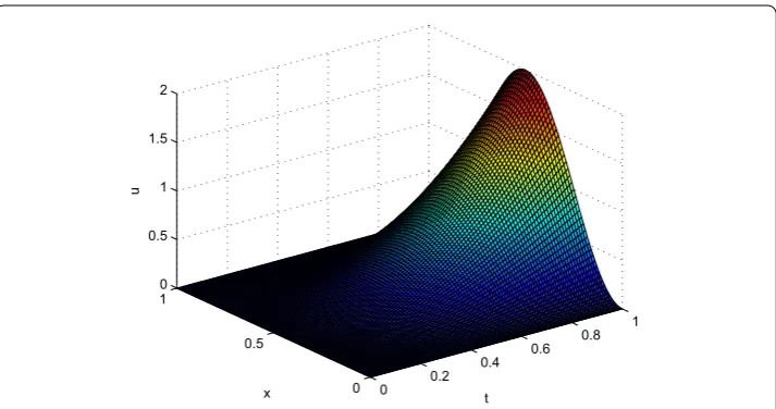
whereα(x,t) = 1 +xt. We take the analytical solutionu(x,t) =t2_{(1 –cos2πx). The behavior}

of the exact solution to equation (53) is shown in Fig.1and the profile of the solution to the fully-discrete form is given in Fig.2.

The numerical solution is in good accordance with the exact solution, indicating that the numerical scheme is valid and efficient.

Then the errors and the orders of convergence are shown in Tables1–3.

5.1 Tables

In Table1, taking the time stept=_200,0001 , we find that the rate of convergence in space is the fourth order in L2 _{norm and is the second order inH}2 _{norm. Tt means that the}

accuracy in space is better than the theoretical precision.

Figure 2The numerical solution to the full-discrete scheme. The figure is the profile of the numerical solution to the cubic B-spline finite element method

Table 1 The error for different space stephatt= 1

(t,h) u–uh Rate u–uh1 Rate u–uh2 Rate

(1/200,000, 1/10) 2.6858e–4 _7.1462e–3 _4.3020e–1

(1/200,000, 1/20) 1.2314e–5 _{4.4470 8.1328e}–4 _{3.1354 1.0389e}–1 _2.0500 (1/200,000, 1/40) 7.4241e–7 _{4.0519 9.9745e}–5 _{3.0274 2.5745e}–2 _2.0127 (1/200,000, 1/80) 4.1905e–8 _{4.1470 1.2399e}–5 _{3.0080 6.4221e}–3 _2.0032

Table 2 The error for different time steptatt= 1

(t,h) u–uh Rate u–uh1 Rate u–uh2 Rate (1/10, 1/800) 5.9048e–4 _2.0970e–3 _1.3459e–2

(1/20, 1/800) 2.7118e–4 _{1.1226 9.6223e}–4 _{1.1239 6.1815e}–3 _1.1225 (1/40, 1/800) 1.3035e–4 _{1.0569 4.6234e}–4 _{1.0574 2.9718e}–3 _1.0566 (1/80, 1/800) 6.4199e–5 _{1.0218 2.2765e}–4 _{1.0221 1.4644e}–3 _1.0210

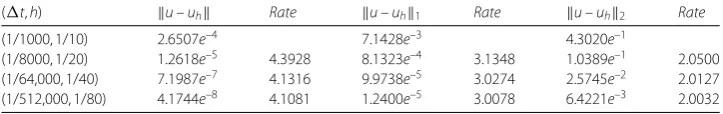
Table 3 The error for different time steptand space stephatt= 1

(t,h) u–uh Rate u–uh1 Rate u–uh2 Rate

(1/1000, 1/10) 2.6507e–4 7.1428e–3 4.3020e–1

(1/8000, 1/20) 1.2618e–5 4.3928 8.1323e–4 3.1348 1.0389e–1 2.0500 (1/64,000, 1/40) 7.1987e–7 4.1316 9.9738e–5 3.0274 2.5745e–2 2.0127 (1/512,000, 1/80) 4.1744e–8 4.1081 1.2400e–5 3.0078 6.4221e–3 2.0032

In Table2, the space step ish=₈₀₀1 . It is easy to see that the orders of error estimate are

O(t) in bothL2_andH2_norms.

In Table3, we choose (t,h) = ( 1 1000,

1 10), (

1 8000,

1 20), (

1 64,000,

1 40), (

1 512,000,

1

80), respectively.

The errors are optimal order convergent inL2_andH2_norms.

The tables show the errors and convergence analysis in space and time. In L2 _norm,

6 Conclusion

In this paper, the model is a class of fourth-order nonlinear parabolic differential equa-tions with variable coefficientα(x,t). By constructing appropriate basis functions satis-fying the boundary conditions, we obtain the finite element schemes based on the cubic B-spline. We analyze the boundedness of the semi-discrete scheme and discuss the er-ror estimates inL2_{norm andH}2_{norm. We also discrete the temporal variable, and the}

fully-discrete scheme is taken as a linearized backward Euler scheme. The coefficient ma-trix of the corresponding linear system is spare, which can be solved efficiently. For the fully-discrete scheme, the rate of convergence is discussed. The numerical results indicate that our method is efficient and its computational accuracy is better than the theoretical results.

Through the above results, we know that the cubic B-splines have better smoothness than the Hermite type elements. The B-spline finite element has only one type of basis functions. It is clear that the B-spline FEM decreases the order of the coefficient matrix, but it can get the same convergence order as the Hermite FEM.

Acknowledgements

The authors would like to express their deep thanks for the referee’s valuable suggestions for the revision and improvement of the manuscript.

Funding

This paper is supported by the Natural Science Foundation of China [grant no. 11561011].

Availability of data and materials Not applicable.

Competing interests

The authors declare that they have no competing interests.

Authors’ contributions

DQ wrote the first draft, made the figure of numerical solution and results on errors, all authors read and approved the final manuscript.

Author details

1_{College of Mathematics, Jilin University, Changchun, P.R. China.}2_{Fundamental Department, Aviation University of Air}

Force, Changchun, P.R. China. 3_{School of Biology and Engineering, Guizhou Medical University, Guiyang, P.R. China.}

Publisher’s Note

Springer Nature remains neutral with regard to jurisdictional claims in published maps and institutional affiliations.

Received: 26 July 2018 Accepted: 19 February 2019 References

1. Hunt, A.W., Orme, C., Williams, D.R.M., Orr, B.G., Sander, L.M.: Instabilities in MBE growth. Europhys. Lett.27(8), 611–616 (1994)

2. Du, Q., Nicolaides, R.A.: Numerical analysis of a continuum model of phase transition. SIAM J. Numer. Anal.28(5), 1310–1322 (1991)

3. Rost, M., Krug, J., Smilauer, P.: Unstable epitaxy on vicinal surfaces. Surf. Sci.369(1), 393–402 (1996) 4. Johnson, M.D., Orme, C., Hunt, A.W., Graff, D., Sudijion, J., Sauder, L.M., Orr, B.G.: Stable and unstable growth in

molecular beam epitaxy. Phys. Rev. Lett.72(1), 116–119 (1994)

5. Rost, M., Krug, J.: Coarsening of surface structures in unstable epitaxial growth. Phys. Rev. E55(4), 3952–3957 (1997) 6. Mullins, W.W.: Flatening of nearly plane surfaces due to capillarity. J. Appl. Phys.30, 77–87 (1959)

7. Krug, J., Plischke, M., Siegert, M.: Surface diffusion currents and the universality classes of growth. Phys. Rev. Lett. 70(21), 3271–3274 (1993)

8. Politi, P., Villain, J.: Ehrlich–Schwoebel instability in molecular-beam epitaxy—a minimal model. Phys. Rev. B54(7), 5114–5129 (1996)

9. Krug, J., Schimschak, M.: Metastability of step flow growth in 1 + 1 dimensions. J. Phys. I5(9), 1065–1086 (1995) 10. Grasselli, M., Mola, G., Yagi, A.: On the longtime behavior of solutions to a model for epitaxial growth. Osaka J. Math.

48(4), 987–1004 (2011)

12. Zhao, X.P., Liu, F.N., Liu, B.: Finite element method for a nonlinear differential equation describing crystal surface growth. Math. Model. Anal.19(2), 155–168 (2014)

13. Ciarlet, P.G.: The Finite Element Method for Elliptic Problems. North-Holland, Amsterdam (1978) 14. Douglas, J., Dupont, T.: Galerkin methods for parabolic equations. SIAM J. Numer. Anal.7, 575–626 (1970) 15. Brenner, S.C., Scott, L.R.: The Mathematical Theory of Finite Element Methods. Springer, Berlin (2002)

16. Chen, H., Chen, Y.: A combined mixed finite element and discontinuous Galerkin method for compressible miscible displacement. SIAM J. Numer. Anal.7, 575–626 (1970)

17. Brezzi, F., Fortin, M.: Mixed and hybrid finite element methods. Natur. Sci. J. Xiangtan Univ.26(2), 119–126 (2004) 18. Choo, S.M., Kim, Y.H.: Finite element scheme for the viscous Cahn–Hilliard equation with a nonconstant gradient

energy coefficient. J. Appl. Math. Comput.19(1–2), 385–395 (2005)

19. Zhang, T.: Finite element analysis for Cahn–Hilliard equation. Math. Numer. Sin.28, 281–292 (2006)

20. Elliott, C.M., French, D.A.: A nonconforming finite element method for the two-dimensional Cahn–Hilliard equation. SIAM J. Numer. Anal.26(4), 889–903 (1989)

21. Barrett, J.W., Blowey, J.F., Garcke, H.: Finite element approximation of a fourth order nonlinear degenerate parabolic equation. Numer. Math.80(4), 525–556 (1998)

22. Kästner, M., Metsch, P., de Borst, R.: Isogeometric analysis of the Cahn–Hilliard equation—a convergence study. J. Comput. Phys.305, 360–371 (2016)

23. Schoenberg, I.J.: Contributions to the problem of approximation of equidistant data by analytic functions. Q. Appl. Math.4, 45–99 (1946)

24. Curry, H.B., Schoenberg, I.J.: On Pólya frequency functions IV: the fundamental spline functions and their limits. J. Anal. Math.17(1), 71–107 (1966)

25. de Boor, C.: B-form basis. In: Farin, G. (ed.) Geometric Modelling, pp. 131–148. SIAM, Philadelphia (1978) 26. de Boor, C., Höllig, K.: Bivariate box splines and smooth pp functions on a three directional mesh. J. Comput. Appl.

Math.9(1), 13–28 (1983)

27. Micchelli, C.A.: A constructive approach to Kergin interpolation inRk_{: multivariateB-splines and Lagrange} interpolation. Rocky Mt. J. Math.10(3), 485–497 (1980)

28. Dahmen, W.: On multivariate B-splines. SIAM J. Numer. Anal.17(2), 179–191 (1980)

29. de Boor, C., de Voer, R.: Approximation by smooth multivariate splines. Trans. Am. Math. Soc.276(2), 131–148 (1983) 30. Cox, M.G.: The numerical evaluation of B-splines. IMA J. Appl. Math.10(2), 134–149 (1972)

31. de Boor, C.: On calculating with B-splines. J. Approx. Theory6(1), 50–62 (1972)

32. Hall, C.A., Meyer, W.W.: Optimal error bounds for cubic spline interpolation. J. Approx. Theory16(2), 105–122 (1976) 33. Hall, C.A.: Natural cubic and bicubic spline interpolation. SIAM J. Numer. Anal.10(6), 1055–1060 (1973)

34. Kolman, R., Okrouhlík, M., Berezovski, A., Gabriel, D., Kopaˇcka, J., Plešek, J.: B-spline based finite element method in one-dimensional discontinuous elastic wave propagation. Appl. Math. Model.46, 382–395 (2017)

35. Soliman, A.A.: A Galerkin solution for Burgers’ equation using cubic B-spline finite elements. Abstr. Appl. Anal.46, 382–395 (2012)

36. Bai, D.M., Zhang, L.M.: The quadratic B-spline finite element method for the coupled Schrodinger–Boussinesq equations. Int. J. Comput. Math.88(8), 1714–1729 (2010)

37. Kutluay, S., Esen, A.: A B-spline finite element method for the thermistor problem with the modified electrical conductivity. Appl. Math. Comput.156(3), 621–632 (2005)

38. Dag, I., Naci Ozer, M.: Approximation of the RLW equation by the least square cubic B-spline finite element method. Appl. Math. Model.25(3), 221–231 (2001)