R E S E A R C H
Open Access
Maximum likelihood estimators of a
long-memory process from discrete
observations
Lin Sun, Lin Wang
*and Pei Fu
*Correspondence:
[email protected] School of Applied Mathematics, Guangdong University of Technology, Guangzhou, P.R. China
Abstract
This paper deals with the problem of estimating the unknown parameters in a long-memory process based on the maximum likelihood method. The mean-square and the almost sure convergence of these estimators based on discrete-time observations are provided. Using Malliavin calculus, we present the asymptotic normality of these estimators. Simulation studies confirm the theoretical findings and show that the maximum likelihood technique can effectively reduce the
mean-square error of our estimators.
MSC: Primary 62D05; secondary 62J12
Keywords: Long-memory processes; Maximum likelihood estimation; Asymptotic analysis; Malliavin calculus
1 Introduction
Brownian motion has been widely used in the Black–Scholes option-pricing framework to model the return of assets. Consequently, several papers have already focused on the valuation of options when the underlying asset of stock price is modeled by a geometric Brownian motion. In this situation, one dimensional distributions of the stock prices are log-normal and the log-returns of the stocks are independent normal random variables. However, empirical studies show that log-returns of financial asset often have the prop-erties of self-similarity and long-range dependency (see Casas and Gao [1]; Los and Yu [2]). To model these observed properties, it is possible to use one of the fractal processes, namely fractional Brownian motion (hereafter fBm), to replace the driving standard Brow-nian motion (see, for example, Willinger et al. [3]). Since fBm is not a semi-martingale (ex-cept in the Brownian motion case), we cannot use the usual stochastic calculus to analyze it. Fortunately, the research was re-encouraged by new insights in stochastic analysis based on the Wick product (see Duncan et al. [4]; Hu and Øksendal [5]), namely the fractional-Itô-integral. Thereafter, many scholars considered the problem of applying fBm in finance in a large setting, such as Elliott and van der Hoek [6]; Elliott and Chan [7]; Guasoni [8]; Rostek [9]; Azmoodeh [10].
When the fBm is used to describe the fluctuation of some financial phenomena, it is important to identify the parameters in stochastic models driven by fBm. This is because all the models involve unknown parameters or functions, which should be estimated from
observations of the process. The estimation of these processes driven by fBm is therefore a crucial step in all applications, particularly in applied finance. For example, a crucial problem with the applications of these option-pricing formulas in the fractional Black– Scholes market in practice is how to obtain the unknown parameters in geometric frac-tional Brownian motion (hereafter gfBm). Otherwise, applying these models with long memory and self-similarity requires efficient and accurate synthesis of discrete gfBm. Even though fBm has stationary self-similar increments, it is neither independent nor Marko-vian. This means that state space models and Kalman filter estimators cannot be applied to the parameters of these processes driven by fBm. However, in the literature, several heuris-tic methods (such as the maximum likelihood approach and the least squares technique) are available to sort out these problems in this kind. For example, several contributions have been already reported for parameter estimation problems concerning continuous-time models where the driving processes are fractional Brownian motions (see Kleptsyna et al. [11]). Actually, the problem of maximum likelihood estimation (hereafter MLE) of the drift parameter has also been extensively studied (see, for example, Kleptsyna and Le Breton [12]; Tudor and Viens [13]). A similar problem for stochastic processes driven by fractional noise in the path-dependent case was investigated in Cialenco et al. [14]. Hu and Nualart [15] obtained least squares estimation (hereafter LSE) for the fractional Ornstein– Uhlenbeck process and proposed the asymptotic normality of LSE using Malliavin calcu-lus. More recently, there has been increased interest in studying asymptotic properties of LSE for the drift parameter in the univariate case with fractional processes (see, Az-moodeh and Morlanes [16]; Cheng et al. [17]). Moreover, Xiao and Yu [18] and Xiao and Yu [19] considered the LSE in fractional Vasicek models in the stationary case, the explo-sive case, and the null recurrent case. For a general theory, including the Girsanov theorem and some results on statistical inference, for finite dimensional diffusions driven by frac-tional noise see also the well summarized monograph by Prakasa Rao [20].
[32] and Bertin et al. [33], who constructed maximum likelihood estimators for both the drift fBm and drift Rosenblatt process. Recently, the parameter estimation problem for the discretely observed fractional Ornstein–Uhlenbeck was studied in Brouste and Iacus [34] and Es-Sebaiy [35]. Kim and Nordman [36] studied a frequency domain bootstrap for approximating the distribution of Whittle estimators for a class of long memory lin-ear processes. Bardet and Tudor [37] presented the theory of the long-memory parameter estimation for non-Gaussian stochastic processes using the Whittle estimator. Xiao et al. [38] used the quadratic variation to estimate unknown parameters of gfBm from discrete observations. In this paper, inspired by Hu et al. [39] and Bertin et al. [32], we estimate the unknown parameters of a special long-memory process with discrete-time data, namely gfBm, based on MLE. The maximum likelihood technique is chosen in this paper because of two reasons: one is that this technique has been applied efficiently in a large set; the other is that it has well-documented favorable properties, such as being asymptotically consistent, unbiased, efficient and normally distributed about the true parameter values. The main contributions of this paper are to determine the estimators for the process of gfBm and to prove the asymptotic properties of these estimators. For these purposes, we first construct estimators of the gfBm, which is observed with random noise errors in the discrete framework. Then we present the asymptotic results. Finally, we perform some simulations in order to study numerically the asymptotic behavior of these estimators.
The remainder of this paper proceeds as follows. Section 2 contains some basic nota-tions on Malliavin calculus that will be used in the forthcoming secnota-tions. Section 3 con-cretely addresses estimators of gfBm. Section 4 deals with the mean-square convergence, the almost surely convergence and the asymptotic normality of these estimators. In Sect. 5, we give simulation examples to show the performance of these estimators, and the stan-dard error is proposed as a criterion of validation. Finally, Sect. 6 makes the concluding remarks. For the sake of the presentation, some difficult technical details are deferred to the Appendix.
2 Preliminaries
In this section we recall some basic results that will be used in this paper and also fix some notations. We refer to Nualart [40] or Hu and Nualart [15] for further reading.
The fBm{BH
t ,t∈R}with the Hurst parameterH∈(0, 1) is a zero mean Gaussian process with covariance
EBHt BHs=RH(s,t) = 1 2
|t|2H+|s|2H–|t–s|2H. (1)
We assume thatBHis defined on a complete probability space (,A,P) such thatAis generated byBH. Fix a time interval [0,T]. Denote byEthe set of real valued step functions on [0,T] and letHbe the Hilbert space defined as the closure ofEwith respect to the scalar product
1[0,t], 1[0,s]H=RH(t,s),
We denote this isometry byϕ−→BH(ϕ). ForH=1
2 we haveH=L2([0,T]), whereas for
H>12 we haveLH1([0,T])⊂Hand forϕ,ψ∈LH1([0,T]) we have
ϕ,ψH=αH T
0
T
0
ϕsψt|t–s|2H–2ds dt, (2)
whereαH=H(2H– 1).
LetSbe the space of smooth and cylindrical random variables in the form of
F=fBH(ϕ1), . . . ,BH(ϕn)
, (3)
wheref ∈Cb∞(Rn) (f and all its partial derivatives are bounded). For a random variableF of the form (3), we define its Malliavin derivative as theH-valued random variable
DF= n
i=1
∂f
∂xi
BH(ϕ1), . . . ,BH(ϕn)
ϕi. (4)
By iteration, one can define themth derivativeDmF, which is an element ofL2(;H⊗m),
for everym≥2. Form≥1,Dm,2denotes the closure ofSwith respect to the norm ·
m,2,
defined by the relation
F2m,2=E|F|2+ m
i=1
EDiF2H⊗i
.
We shall make use of the following theorem for multiple stochastic integrals (see Nualart and Peccati [41] or Nualart and Ortiz-Latorre [42]).
Theorem 2.1 Let Fn,n≥1be a sequence of random variables in the pth Wiener chaos,
p> 2,such thatlimn→∞E(Fn2) =σ2.Then the following conditions are equivalent:
(i) Fnconverges in law toN(0,σ2)asntends to infinity;
(ii) DFn2Hconverges inL2to a constant asntends to infinity.
Remark2.2 In Nualart and Ortiz-Latorre [42], it is proved that (i) is equivalent to the fact thatDFn2H converges inL2topσ2asntends to infinity. If we assume (ii), the limit of DFn2Hmust be equal topσ2because
EDFn2H
=pEFn2.
3 Maximum likelihood estimators
In the literature, it is common to use the following form to model the underlying asset priceStof a derivative:
dSt=μStdt+σStdBHt , t≥0, (5)
whereμ,σ andHare constants to be estimated, and (BH
Hence the parameter estimation is an important problem. Using the Wick integration, Hu and Øksendal [5] stated that the solution of (5) is
St=S0exp μt–
1 2σ
2t2H+σBH t
, t≥0. (6)
Hence, estimating the parameters in (5) is equal to estimate the parameters from the following model:
Xt=μt– 1 2σ
2t2H+σBH
t , t≥0. (7)
Letμ=a, –12σ2=bandσ=c. Then we consider a general model as follows:
Yt=at+bt2H+cBHt , t≥0. (8)
We assume that the process is observed at discrete-time instants (t1,t2, . . . ,tN). This is a natural situation that one encounters in practice. In this situation, we have a sample of discrete observations and try to estimate parameters for the process of (8) generating the sample. In the case of stochastic processes driven by Brownian motion, this problem have been well studied. The Markov structure of Brownian motion is essential for most of the methods used and therefore studying this problem in non-Markovian models seems chal-lenging in this paper. On the other hand, for Gaussian processes estimation techniques have been quite extensively developed and it becomes apparent that some of these tech-niques work fine for an estimation of the unknown parameters for the process of (8). The reasons why we do not use the likelihood given by the Girsanov transformation for es-timating the unknown parameters (Cialenco et al. [14]) are twofold. First of all, the Gir-sanov transformation gives the likelihood for continuous observations of the process. In practice we have discrete observations so we need to approximate the integrals appearing in the likelihood by discrete analogs. This requires the time between observations to be small, which is not always the case. Furthermore, the Girsanov transformation gives the likelihood as a function ofaandb. It cannot provide us with insights for estimatingH, which in most practical situations will be unknown. This differs from the classical case where H= 1/2 is known. Hence, although the Girsanov transformation is theoretically interesting, it does not seem very practical to use it in the context of parameter estima-tion for the process (8). Consequently, our technic used in this paper is inspired from Hu et al. [39], which seems the best way to estimate (8). To simplify notations, we as-sumetk=kh,k= 1, 2, . . . ,N, for some fixed lengthh> 0. Thus the observation vector is
Y= (Yh,Y2h, . . . ,YNh)(where the superscriptdenotes the transpose of a vector). There are two reasons for us to study the general case of (8). One is because we can obtain the explicit estimators. The other is that it is also widely applied in various fields. The loga-rithm of a widely used gfBm, which is popular in finance (see Hu and Øksendal [5]), is of the form (8). Moreover, the motivation of the model of (8) is the extension of gfBm. Now, we introduce the following notations:
Y=at+bt2H+cBHt , (9)
where t = (h, 2h, . . . ,Nh), t2H= (h2H, (2h)2H, . . . , (Nh)2H)and BH
First, let us discuss the estimation of the Hurst parameter in the model (9). From Corol-lary 2 in Kubilius and Melichov [43], we immediately obtain the estimator ofHfrom the observation Y:
wherezdenotes the greatest integer not exceedingz.
Thus it is easy to obtain an estimator for the Hurst parameter by using such quadratic variations. Moreover, using the same argument of Kubilius and Melichov [43], we find that the estimatorHˆ (defined by (10)) is a strong consistent estimator ofHasNgoes to infinity. Essentially, the problem of estimating the Hurst parameter in fractional processes has been extensively studied (see Shen et al. [44]; Kubilius and Mishura [45]; Salomónab and Fortc [46]). Therefore, throughout this paper, we assume that the Hurst coefficient is known. Thus, the aim of this paper is to estimate the unknown parametersa,bandc2
from observationsY=Yih, 0≤i≤N, for a fixed intervalhand study their asymptotic properties asN→ ∞.
Actually, as the law of Y is Gaussian, the likelihood function of Y can be explicitly eval-uated. Thus the estimators ofa,bandc2can be provided by the following theorem.
Theorem 3.1 The maximum likelihood estimators of a,b and c2from the observationY
are given by
Proof Since Y is Gaussian, the joint probability density function of Y is
gY;a,b,c2=2πc2–N2|
Then we obtain the log-likelihood function
The MLE of a, b and c2 are obtained by maximizing the log-likelihood function
L(Y;a,b,c2) with respect to a, b and c2, respectively. Finally, we obtain (11), (12)
and (13).
4 The asymptotic properties
In this section we will discuss theL2-consistency, the strong consistency and the
asymp-totic normality for the MLEs ofa,bandc2.
First, we consider theL2-consistency of (11) and (12).
Theorem 4.1 Both MLEs of a(defined by(11))and b(defined by(12))are unbiased and
Thusaˆis unbiased. On the other hand, using (15), we have
Circle Theorem (see Golub and van Loan [47]: Theorem 8.1.3, p. 395)
λmax(H)≤ max
i=1,...,N N
j=1
|ij| ≤CN2H+1,
whereCis a positive constant. Thus we have
tH–1t≥CN2–2H. (16)
Moreover, a similar computation, combined with Theorem 1 of Zhan [48], implies that
(tH–1t2H)2
(t2H)–1
Ht2H
≤ λmax(H) 14H+ 24H+· · ·+N4H
11+2H+ 21+2H+· · ·+N1+2H λmin(H)
2
≤ ˆCN6–2H, (17)
withCˆ a positive constant.
Consequently, using (16) and (17), we see thatVar[aˆ] converges to zero asN→ ∞. In
the same way we can prove the convergence ofbˆ.
In what follows, we study the mean-square convergence of the estimatorcˆ2defined by (13).
Theorem 4.2 The estimatorcˆ2(defined by(13))of c2has “normal” N–2
N bias and it
con-verges in mean square to c2as N→ ∞.That is to say,
Eˆc2=N– 2
N c
2 and Varˆc2−−−→N→∞ 0. (18)
Proof By replacing Y withat+bt2H+cBH
t in (13), we have
ˆ
c2=c
2
N
BHt H–1BHt – 1
t–1Ht·(t2H)–1
Ht2H– (tH–1t2H)2 ·BHt –1Ht2H2·t–1Ht+tH–1BHt 2·t2HH–1t2H
– 2·t–1Ht2H·t–1HBHt ·t2HH–1BHt . (19)
Now, using (28) in the Appendix we have
Eˆc2=N– 2
N c
4.
Finally, using (28) and (29) in the Appendix, we have
Varcˆ2=Ecˆ22–Eˆc22=2c
2
N ,
which is convergent to 0 asNgoes to infinity. Thus we proved the theorem.
Theorem 4.3 The estimatorsaˆ,b andˆ cˆ2 defined by(12), (13)and(14),respectively,are
strongly consistent,that is,
ˆ
a→a a.s. as N→ ∞, (20)
ˆ
b→b a.s. as N→ ∞, (21)
ˆ
c2→c2 a.s. as N→ ∞. (22)
Proof First, we will discuss the convergence ofaˆ. To this end, we will show that
N≥1
P |ˆa–a|> 1
N
<∞, (23)
for some> 0.
Take 0 << 1 –H. Since the random variableaˆ–ais a Gaussian random variable, from Chebyshev’s inequality and the property of the central absolute moments of Gaussian ran-dom variables, we have
P |ˆa–a|> 1
N
≤NqE|ˆa–a|q≤CqNq
E|ˆa–a|2q/2
≤Cqσqh(H–1)qNq+(H–1)q,
whereCqis a constant depending onq. For sufficiently largeq, we haveq+ (H– 1)q< –1. Thus (23) is proved, which implies (20) by the Borel–Cantelli lemma.
Moreover, (21) and (22) can be obtained in a similar way.
Now we are in the position to present the asymptotic normality for the estimatorsaˆ,bˆ
andˆc2. First from (15), it is clear that
t–1Ht– (t –1
Ht2H)2 (t2H)–1
Ht2H
(aˆ–a)−→L N0,c2 asNtends to infinity,
where−→L denotes convergence in the distribution. Similarly, we obtain
t–1Ht– (t –1
Ht2H)2 (t2H)–1
Ht2H
(bˆ–b)−→L N0,c2 asNtends to infinity.
Hence, only the asymptotic distribution ofˆc2is left to be studied in the following
theo-rem.
Theorem 4.4 The estimatorˆc2(defined by(14))of c2is asymptotic normality.That is to say,
1
c2
N
2
ˆ
Proof Using (19), we can define
From (28) and (29) in the Appendix, we can show that
lim
From Theorem 4 in Nualart and Ortiz-Latorre [42] (see also Theorem 2.1 in Sect. 2), in order to show (24), it suffices to show thatDFN2Hconverges to a constant inL2asN tends to infinity. Using (4), we can obtain
we have shown thatDFN2H converges to a constant inL2asN tends to infinity. This
completes the proof of this theorem.
5 Simulation
In this section, we construct Monte Carlo studies for the different values ofa,bandc2to
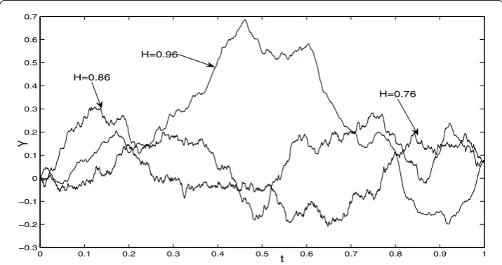
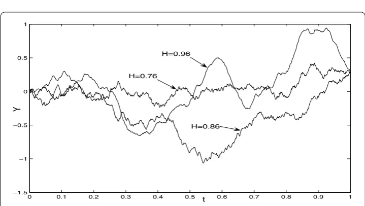
numerically investigate the efficiency of our estimators. Actually, the main obstacle to a Monte Carlo simulation is to obtain fBm, in contrast to the standard Brownian motion. However, in the literature, there are alternative methods to solve this problem (see Coeur-jolly [49]). In this paper, we use Paxson’s algorithm (see Paxson [50]). First, we generate fractional Gaussian noise based on Paxson’s method by fast Fourier transformation. Sec-ond, we obtain the fBm using the result that a fBm is defined as the partial sum of the fractional Gaussian noise. Finally, we obtain the process of (9). ForN= 1000,h= 0.001 andt∈[0, 1], some sample trajectories of the process (9) are shown Figs. 1–3 for different values ofH,a,bandc2. The simulation results reflex main properties of fBm: a larger value
ofHcorresponds to smoother sample paths.
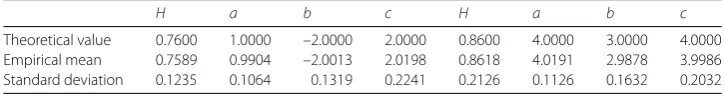
In the following, we consider the problem of estimatingH,a,bandcfrom the obser-vationsYh, . . . ,YNh. We have simulated the observationsYh, . . . ,YNhfor different values of
H, a,b andcwith the steph= 0.01. For each case we simulate the observations (N is presented in the following tables) and calculate 80 estimation of estimators. Then we can implement the observations to obtain the estimators by an exact MLE method. The sim-ulated mean and variance of these estimators are given in the following tables (true value is the parameter value used in the Monte Carlo simulation; the empirical mean and the standard deviation are for the sample statistics).
From the output of the numerical computations, we find that both the standard devi-ations and the absolute errors ofH,a,bandcdecrease to zero as the number of obser-vations increases. The computation results demonstrate that the simulated mean of the maximum likelihood estimators converges to the true value rapidly. Hence we can see that the estimators are excellent forH>12. In summary, our estimation results also show that
Figure 2Sample paths of model (9) for different values of Hurst parameter (Chosen parametersa= 0.25; b= 0.45;c= 0.3)
Figure 3Sample paths of model (9) for different values of Hurst parameter (Chosen parametersa= 0.36; b= 0.28;c= 0.40)
the MLE performs well since the estimating results match the chosen parameters exactly. Comparing the results of Tables 1–3 above with those of Tables 1–3 in Hu et al. [39], we can see that the standard deviation is considerably larger than those of Hu et al. [39]. The reason for this difference is that the authors assumed that the Hurst parameter was known in Hu et al. [39]. Our estimators ofa,bandcin this paper include the estimator ofH. It is worth to emphasize that a bad estimate ofHmay lead to a poor estimate ofa,bandc. Obviously, more accuracy of the estimator forHleads the small standard deviation. Let us also mention that the accuracy of the estimator forHcan affect the accuracy ofa,b
Table 1 The means and standard deviations of the estimators withN= 600
H a b c H a b c
Theoretical value 0.7600 1.0000 –2.0000 2.0000 0.8600 4.0000 3.0000 4.0000 Empirical mean 0.7497 1.1264 –2.1076 2.1233 0.8701 3.9068 3.1098 3.9098 Standard deviation 0.6573 0.6866 0.5298 0.5290 0.5508 0.6109 0.5604 0.6533
Table 2 The means and standard deviations of the estimators withN= 900
H a b c H a b c
Theoretical value 0.7600 1.0000 –2.0000 2.0000 0.8600 4.0000 3.0000 4.0000 Empirical mean 0.7511 1.0976 –2.0916 2.0876 0.8678 4.0617 2.9356 3.9433 Standard deviation 0.3546 0.3325 0.4893 0.4729 0.4675 0.4667 0.3984 0.4625
Table 3 The means and standard deviations of the estimators withN= 1200
H a b c H a b c
Theoretical value 0.7600 1.0000 –2.0000 2.0000 0.8600 4.0000 3.0000 4.0000 Empirical mean 0.7589 0.9904 –2.0013 2.0198 0.8618 4.0191 2.9878 3.9986 Standard deviation 0.1235 0.1064 0.1319 0.2241 0.2126 0.1126 0.1632 0.2032
6 Conclusion
The processes of long memory have evolved into a vital and important part of the time se-ries analysis during the last decades, as studies in empirical finance have sought to use the “ideal” models in practical applications of importance in the financial engineering. Among them, the gfBm has been shown by many authors to be a useful description of financial time series. However, when employing a continuous mathematical framework to discrete data, it is important to provide optimal methods for estimating the correct parameters of this process. In this paper, we have extended the notion of gfBm into the discrete do-main and then proposed the methodology of parameter estimation in time series driven by gfBm. For these purposes we construct the estimators by MLE and provide the conver-gence analysis for these estimators. Moreover, numerical study illustrated the effective-ness of the methodology. As can be seen in Tables 1–3, the MLE provides a mean which is consistent with the true value and presents a variance which is nearly equal to zero. Hence the numerical results show that the MLE is a fast, accurate and reliable methodol-ogy to estimate the parameters of gfBm. Although in the present paper we only develop the asymptotic theory for a special linear long memory model driven by fBm, our method is generally applicable to discrete-time models with a linear drift and with a constant dif-fusion, which are driven by centered Gaussian processes. Furthermore, we can see that model (9) can be considered as a general model of long memory property. It is obvious that some interesting cases are included in (9). In particular:
(i) Whenb= 0, we can obtain the fBm with drift parameter. (ii) ForH=12, we can obtain the geometric Brownian motion. (iii) IfH=1
2,c= 1andb= 0, we can get the linear regression model.
(iv) Ifb= 0andc= 1, we can get the regression model with long-memory errors.
in the statistical machinery that is available to practitioners to grow further as the finan-cial industry continues to expand and data sets become richer. The field is therefore of growing importance for both theorists and practitioners.
Appendix
In this appendix we show how to obtain the required moment computation forcˆ2.
Proposition 7.1 Letcˆ2be defined by(13).Then
Eˆc2=N– 2
N c
2, (28)
Eˆc4=N
2– 2N+ 4
N2 c
4. (29)
Proof First, using Theorem 10.18 in Schott [51],E[(BH
t BHt )] =Hand (19), we can com-pute the expectation ofcˆ2as follows:
Eˆc2=c
2
N
EBHt –1HBHt – 1
t–1Ht·(t2H)–1
Ht2H– (tH–1t2H)2
·t2HH–1EBtHBHt H–1t2H·tH–1t+ t–1HEBHt BHt –1Ht
·t2HH–1t2H– 2·tH–1t2H·tH–1EBHt BHt H–1t2H
=N– 2
N c
2.
To compute the variance ofcˆ2, we introduce X =–1/2
H (BHt ). Then
EXX=EH–1/2BtHBHt –1/2H =I.
Therefore, X is a standard Gaussian vector of dimensionN. For anyλsmall enough and ε∈R, we have
EexpλBHt H–1BHt +εtH–1BHt
=Eexpλ|X|2+εt–
1 2
H X
= 1
(2π)N2
RN e–|X|
2
2 +λX2+εt – 12
H XdX.
A standard technique of completing the squares yields
EexpλBHt H–1BHt +εtH–1BHt )
= (1 – 2λ)–N2 exp
ε2t–1Ht
2(1 – 2λ)
What we are only interested are the coefficients ofλ2,λε2andε4in the above expression
f(λ,ε). We have
f(λ,ε) =1 +Nλ+N(N+ 2)λ2+· · ·1 +ε
2t–1
Ht
2 (1 + 2λ+· · ·) +· · ·
.
Comparing the coefficients ofλ2,λε2andε4, we have
EBHt H–1BHt 2=N(N+ 2),
EBHt H–1BHt t–1HBHt 2= (N+ 2)t–1Ht, Et–1HBHt 4= 3tH–1t.
Then we can obtain
EBHt H–1BHt t2H–1HBHt 2= (N+ 2)t2HH–1t2H, Et2HH–1BHt 4= 3t2HH–1t2H.
Analogously to the discussion above, we obtain
Eˆc4= c
4
N2E
BHt –1HBHt – 1
t–1Ht·(t2H)–1
Ht2H– (tH–1t2H)2 ·BHt H–1t2H2·tH–1t+t–1HBHt 2·t2H–1Ht2H
– 2·tH–1t2H·tH–1BHt ·t2H–1HBHt
2
=N
2– 2N+ 4
N2 c
4,
which completes the proof.
Acknowledgements
The author would like to thank the referees for their very helpful and detailed comments, which have significantly improved the presentation of this paper.
Funding
This research was supported by the Natural Science Foundation of Guangdong Province, China (no. S2013010016270).
Competing interests
The authors declare that they have no competing interests.
Authors’ contributions
LS carried out the proofs of all theorems. LW participated in the design of the study and helped to draft the manuscript. PF conceived of the Monte Carlo simulation study. All authors contributed equally and significantly in writing this article. All authors read and approved the final manuscript.
Publisher’s Note
Springer Nature remains neutral with regard to jurisdictional claims in published maps and institutional affiliations.
References
1. Casas, I., Gao, J.: Econometric estimation in long-range dependent volatility models: theory and practice. J. Econom.
147(1), 72–83 (2008)
2. Los, C.A., Yu, B.: Persistence characteristics of the Chinese stock markets. Int. Rev. Financ. Anal.17(1), 64–82 (2008) 3. Willinger, W., Taqqu, M.S., Teverovsky, V.: Stock market prices and long-range dependence. Finance Stoch.3(1), 1–13
(1999)
4. Duncan, T.E., Hu, Y., Pasik-Duncan, B.: Stochastic calculus for fractional Brownian motion I: theory. SIAM J. Control Optim.38(2), 582–612 (2000)
5. Hu, Y., Øksendal, B.: Fractional white noise calculus and applications to finance. Infin. Dimens. Anal. Quantum Probab. Relat. Top.6(1), 1–32 (2003)
6. Elliott, R.J., van der Hoek, J.: A general fractional white noise theory and applications to finance. Math. Finance13(2), 301–330 (2003)
7. Elliott, R.J., Chan, L.: Perpetual American options with fractional Brownian motion. Quant. Finance4(2), 123–128 (2004)
8. Guasoni, P.: No arbitrage under transaction costs, with fractional Brownian motion and beyond. Math. Finance16(3), 569–582 (2006)
9. Rostek, S.: Option Pricing in Fractional Brownian Markets. Springer, Heidelberg (2009)
10. Azmoodeh, E.: On the fractional Black–Scholes market with transaction costs. Commun. Math. Finance2(3), 21–40 (2013)
11. Kleptsyna, M.L., Le Breton, A., Roubaud, M.C.: Parameter estimation and optimal filtering for fractional type stochastic systems. Stat. Inference Stoch. Process.3(1), 173–182 (2000)
12. Kleptsyna, M.L., Le Breton, A.: Statistical analysis of the fractional Ornstein–Uhlenbeck type process. Stat. Inference Stoch. Process.5(3), 229–248 (2002)
13. Tudor, C.A., Viens, F.: Statistical aspects of the fractional stochastic calculus. Ann. Stat.25(5), 1183–1212 (2007) 14. Cialenco, I., Lototsky, S., Pospisil, J.: Asymptotic properties of the maximum likelihood estimator for stochastic
parabolic equations with additive fractional Brownian motion. Stoch. Dyn.9(2), 169–185 (2009)
15. Hu, Y., Nualart, D.: Parameter estimation for fractional Ornstein–Uhlenbeck processes. Stat. Probab. Lett.80(11–12), 1030–1038 (2010)
16. Azmoodeh, E., Morlanes, J.I.: Drift parameter estimation for fractional Ornstein–Uhlenbeck process of the second kind. Statistics49(1), 1–18 (2015)
17. Cheng, P., Shen, G., Chen, Q.: Parameter estimation for nonergodic Ornstein–Uhlenbeck process driven by the weighted fractional Brownian motion. Adv. Differ. Equ.2017, 366 (2017)
18. Xiao, W., Yu, J.: Asymptotic theory for estimating drift parameters in the fractional Vasicek model. Econ. Theory (2018) (forthcoming)
19. Xiao, W., Yu, J.: Asymptotic Theory for Rough Fractional Vasicek Models. Economics and Statistics Working Papers 7-2018, Singapore Management University, School of Economics (2018).
http://ink.library.smu.edu.sg/soe_research/2158
20. Prakasa Rao, B.L.S.: Statistical Inference for Fractional Diffusion Processes. Wiley, New York (2010)
21. Xiao, W., Zhang, W., Xu, W.: Parameter estimation for fractional Ornstein–Uhlenbeck processes at discrete observation. Appl. Math. Model.35(9), 4196–4207 (2011)
22. Long, H., Shimizu, Y., Sun, W.: Least squares estimators for discretely observed stochastic processes driven by small Lévy noises. J. Multivar. Anal.116(1), 422–439 (2013)
23. Liu, Z., Song, N.: Minimum distance estimation for fractional Ornstein–Uhlenbeck type process. Adv. Differ. Equ.
2014(1), 137 (2014)
24. Barboza, L.A., Viens, F.G.: Parameter estimation of Gaussian stationary processes using the generalized method of moments. Electron. J. Stat.11(1), 401–439 (2017)
25. El Onsy, B., Es-Sebaiy, K., Viens, F.G.: Parameter estimation for a partially observed Ornstein–Uhlenbeck process with long-memory noise. Stochastics89(2), 431–468 (2017)
26. Bajja, S., Es-Sebaiy, K., Viitasaari, L.: Least squares estimator of fractional Ornstein–Uhlenbeck processes with periodic mean. J. Korean Stat. Soc.46(4), 608–622 (2017)
27. Fox, R., Taqqu, M.S.: Large-sample properties of parameter estimates for strongly dependent stationary Gaussian time series. Ann. Stat.14(2), 517–532 (1986)
28. Dahlhaus, R.: Efficient parameter estimation for self-similar processes. Ann. Stat.17(4), 1749–1766 (1989) 29. Tsai, H., Chan, K.S.: Quasi-maximum likelihood estimation for a class of continuous-time long-memory processes.
J. Time Ser. Anal.26(5), 691–713 (2005)
30. Tsai, H., Chan, K.S.: Maximum likelihood estimation of linear continuous time long memory processes with discrete time data. J. R. Stat. Soc. B67(5), 703–716 (2005)
31. Bhansali, R.J., Giraitis, L., Kokoszka, P.: Estimation of the memory parameter by fitting fractionally differenced autoregressive models. J. Multivar. Anal.97(10), 2101–2130 (2006)
32. Bertin, K., Torresa, S., Tudor, C.A.: Maximum likelihood estimators and random walks in long memory models. Statistics45(4), 361–374 (2011)
33. Bertin, K., Torres, S., Tudor, C.A.: Drift parameter estimation in fractional diffusions driven by perturbed random walks. Stat. Probab. Lett.81(2), 243–249 (2011)
34. Brouste, A., Iacus, S.M.: Parameter estimation for the discretely observed fractional Ornstein–Uhlenbeck process and the Yuima R package. Comput. Stat.28(4), 1529–1547 (2013)
35. Es-Sebaiy, K.: Berry–Esséen bounds for the least squares estimator for discretely observed fractional Ornstein–Uhlenbeck processes. Stat. Probab. Lett.83(10), 2372–2385 (2013)
36. Kim, Y.M., Nordman, D.J.: A frequency domain bootstrap for Whittle estimation under long-range dependence. J. Multivar. Anal.115, 405–420 (2013)
37. Bardet, J.M., Tudor, C.: Asymptotic behavior of the Whittle estimator for the increments of a Rosenblatt process. J. Multivar. Anal.131, 1–16 (2014)
39. Hu, Y., Nualart, D., Xiao, W., Zhang, W.: Exact maximum likelihood estimator for drift fractional Brownian motion at discrete observation. Acta Math. Sci.31(5), 1851–1859 (2011)
40. Nualart, D.: The Malliavin Calculus and Related Topics, 2nd edn. Springer, Berlin (2006)
41. Nualart, D., Peccati, G.: Central limit theorems for sequences of multiple stochastic integrals. Ann. Probab.33(1), 177–193 (2005)
42. Nualart, D., Ortiz-Latorre, S.: Central limit theorems for multiple stochastic integrals and Malliavin calculus. Stoch. Process. Appl.118(4), 614–628 (2008)
43. Kubilius, K., Melichov, D.: Quadratic variations and estimation of the Hurst index of the solution of SDE driven by a fractional Brownian motion. Lith. Math. J.50(4), 401–417 (2010)
44. Shen, H., Zhu, Z., Lee, L.T.C.: Robust estimation of the self-similarity parameter in network traffic using wavelet transform. Signal Process.87(9), 2111–2124 (2007)
45. Kubilius, K., Mishura, Y.: The rate of convergence of Hurst index estimate for the stochastic differential equation. Stoch. Process. Appl.122(11), 3718–3739 (2012)
46. Salomónab, L.A., Fortc, J.C.: Estimation of the Hurst parameter in some fractional processes. J. Stat. Comput. Simul.
83(3), 542–554 (2013)
47. Golub, G.H., van Loan, C.F.: Matrix Computations, 3rd edn. Johns Hopkins University Press, Baltimore (1996) 48. Zhan, X.: Extremal eigenvalues of real symmetric matrices with entries in an interval. SIAM J. Matrix Anal. Appl.27(3),
851–860 (2005)
49. Coeurjolly, J.F.: Simulation and identification of the fractional Brownian motion: a bibliographical and comparative study. J. Stat. Softw.5(7), 1–53 (2000)
50. Paxson, V.: Fast, approximate synthesis of fractional Gaussian noise for generating self-similar network traffic. Comput. Commun. Rev.27(5), 5–18 (1997)