R E S E A R C H
Open Access
A distributed broadcast algorithm for
duty-cycled networks with physical
interference model
Dianbo Zhao and Kwan-Wu Chin
*Abstract
Broadcast is a fundamental operation in multi-hop wireless networks. Given a source node with a message to broadcast, the objective is to propagate the message to all nodes in an interference-free manner while incurring minimum latency. This problem, called Minimum-Latency Broadcast Scheduling (MLBS), has been studied extensively in wireless networks whereby nodes remain on all times and has been shown to be NP-hard. However, only a few studies have addressed this problem in the context of duty-cycled wireless networks, which unfortunately, remains NP-hard. In these networks, nodes do not wake up simultaneously, and hence, not all neighbors of a transmitting node will receive a broadcast message at the same time, meaning multiple transmissions may be necessary. Moreover, most of these studies addressed the MLBS problem over the idealistic protocol interference model. Henceforth, this paper considers MLBS for duty-cycled wireless networks under the physical interference model and presents an approximation algorithm called hexagon-based broadcast algorithm (HBA), which has a constant ratio in terms of broadcast latency and transmission times. We have evaluated HBA in different network configurations, and the results show that the latencies achieved by our algorithm are much lower than existing schemes. In particular, HBA manages to half the broadcast latency achieved by the state-of-the-art tree-based algorithm.
Keywords: Duty-cycled networks; Physical interference model; Distributed broadcast; Minimum latency
1 Introduction
Wireless sensor networks (WSNs) consist of numerous nodes deployed in a field. These nodes may be resource constrained in terms of battery lifetime, memory, and processor speed. In addition, they use multi-hop commu-nications whereby sensed data are forwarded to one or more sinks/gateways via one or more nodes. Upon receiv-ing the data, a sink/gateway may transmit a command to sensor nodes to affect their operating parameters; e.g., sampling frequency. Consequently, network-wide broad-cast from a sink is a fundamental operation. Apart from that, broadcast is relied upon by several network proto-cols, such as routing [1], information dissemination [2], and resource/service discovery [3]. These protocols in turn help applications in disaster relief, military commu-nication, rescue operation, and object detection [4].
*Correspondence: [email protected]
School of Electrical, Computer and Telecommunications Engineering, University of Wollongong, Wollongong 2500, Australia
For these applications, time is critical, and hence, a Minimum-Latency Broadcast Scheduling (MLBS) algo-rithm/protocol will be of great importance to their oper-ation. Like many other communication protocols, any developed MLBS solution must deal with interference. Unfortunately, the MLBS problem for multi-hop wire-less networks has been proven to be NP-hard [5], and researchers have proposed many approximation algo-rithms; see [4-10]. These algorithms, however, assume all nodes are always active and adopt highly theoretical disk graph models, in which the transmission and inter-ference range is assumed to be a unit disk centered at each node. These works deal with interference through the RTS/CTS model or protocol interference model [11]. RTS/CTS model only considers the interference within a node’s transmission range; that is, interference and trans-mission range are equal. On the other hand, the protocol interference model assumes that the interference range is larger than transmission range. Specifically, interference is assumed when nodes have overlapping interference range.
These ‘interfered nodes’ must therefore be scheduled in different time slots. The main drawback of these inter-ference models is that they cannot model the case where many far-away nodes could still have non-negligible effect on reception. To this end, the physical interference model, also called SINR-based interference model, is more real-istic, where the cumulative interference of many nodes outside the interference range is not neglected.
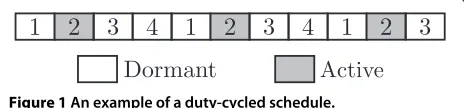
To date, only a few broadcast algorithms [7,12,13] have been designed for the MLBS problem under the physical interference model. Notably, there are even fewer works that address the MLBS problem in duty-cycled wireless networks. Briefly, in these networks, nodes are powered by batteries and are only awake for a fraction of the time [14]. Here, the duty cycle of a node is defined as the ratio between its active time and scheduling period, denoted asT. We note that they can employ a synchronous wake-up schedule; that is, nodes wake wake-up at the same time. This means existing MLBS solutions for always on nodes are applicable. Unfortunately, doing so would require sen-sor nodes to coordinate and synchronize their wake-up time globally. This incurs high signaling overheads and energy that may severely shorten their operational life-time. This paper, therefore, only considers wireless net-works with an asynchronous schedule. Advantageously, Chin [15] showed that nodes only need to maintain the clock offset to each neighbor. To reduce signaling over-heads even further, nodes can select a random sequence of wake-up times independently instead of having a coor-dinated wake-up schedule, which requires network-wide negotiation, where all nodes are awake. Figure 1 shows a sequence of four slots that repeat periodically. The grayed slots denote the wake-up times of a node. In this exam-ple, the node has picked slot ‘2’ as its active time slot from a scheduling periodT of 4, and hence, its duty cycle is 14. In fact, in a duty-cycled WSN, all nodes will pick their own wake-up time upon network boot-up; in this example, a random slot in the range [1,4]. Once selected, a node then wakes up in its chosen slot every T slots. Given the wake-up schedule of nodes, a broadcasting node may have to transmit a message multiple times; i.e., all neighbors are unlikely to select the same slot to wake up. Consequently, any solutions to the MLBS problem in duty-cycled networks must first determine the wake-up times of neighbors, and in each wake-up time, it needs to ensure transmissions do not collide.
Figure 1An example of a duty-cycled schedule.
Henceforth, this paper presents the design and evalua-tion of a novel approximaevalua-tion algorithm that is designed for duty-cycled networks under the physical interference model. Specifically, it contains the following contribu-tions:
1. We propose the first distributed broadcast algorithm, called hexagon-based broadcast algorithm (HBA), for the problem at hand. It produces a constant
approximation ratioaof
9
2+231−(r8/rβ
max)α
2
α−2+α−11+3
1/α2 Tin
terms of broadcast latency, whereαis the path-loss exponent,βis the minimum SINR threshold required for a message to be decoded successfully,rmaxis the maximum transmission range,ris the transmission range of nodes, andTis the scheduling period. 2. The total number of transmissions in terms of
broadcast messages produced by HBA is upper-bounded by(T+1)NH, whereNHis the number of hexagons required to cover the entire network. 3. We evaluate HBA under different network
parameters via simulation and show that that on average, our proposed algorithm has a much better performance in terms of broadcast latency than the tree-based algorithm [7]. The key reason is because our algorithm is able to schedule transmissions in multiple layers as opposed to layer by layer, as is done by [7].
The remainder of this paper is organized as follows. Section 2 lists related work. In Section 3, we introduce the network model, definitions, theories, and the problem for-mulation. In Section 4, we introduce our approximation algorithm, followed by its analysis in Section 5. Section 6 presents our research methodology and results. Lastly, Section 7 concludes the paper and presents future works.
2 Related works
To date, there are many approaches to address the MLBS problem in multi-hop wireless networks. The simplest by far is flooding [16], where each node simply re-transmits a received message to its neighbors unscrupulously. How-ever, this causes broadcast storms [17] and is thus very costly and causes long latencies. Consequently, a num-ber of researchers, e.g., [18-20], have proposed methods that improve the efficiency of broadcast. In this paper, we address a variant of the MLBS problem, which aims to find an efficient, interference-free schedule that yields the minimum broadcast latency.
constant approximation ratio of more than 400 for one-to-all broadcast. They then improve this ratio to 12 in [4]. Huang et al. [8] outlined three approximation algo-rithms for MLBS with latency of at most 24R, 16R, and
R+O(log2R), respectively, and the omitted constant in O(log2R)exceeds 150 [4], whereRis the theoretical lower-bound.
To the best of our knowledge, Chen et al. [6] are the first to study the MLBS problem under the protocol interfer-ence model, where the interferinterfer-ence range is larger than transmission range. Huang et al. [7] propose a constant approximation algorithm with a ratio of 623(+2)2 for the MLBS problem, where is the ratio between the interference range and transmission range. Tiwari et al. [10] extend Huang et al.’s method to consider different transmission ranges and dimensions, i.e., 2D and 3D, and presented an approximation algorithm with a constant ratio of24
3(+1)2γ2+ 8γ (+1)
3 +43 for the 2D space, where
γ is the ratio between the maximum and minimum trans-mission range. Tiwari et al. [10] also propose the first distributed algorithm for the MLBS problem under the protocol interference model. However, their distributed algorithm requires a node to exchange a significant num-ber of control messages until all its neighbors receive the broadcast message, leading to an increase in energy con-sumption. Mahjourian et al. [9] study the conflict-aware broadcast problem whereby apart from the transmission and interference range, they also consider the carrier sensing range. They propose a constant approximation algorithm that has a ratio of O(max(,δ)2), where δ is the approximation ratio between the carrier sensing and transmission range.
There are only handful works that have considered the MLBS problem with the physical interference model. Huang et al. [7] propose the first approximation algorithm for the MLBS problem under the physical interference model assuming each node is aware of its geographi-cal location. Wan et al. [13] convert the network under the physical interference model into a disk graph and apply coloring methods to schedule simultaneous trans-missions. Huang et al. [12] then extend the approach in [7] to consider a more realistic interference model, where a message is received successfully as per its SINR level.
Thus far, the aforementioned works assume an always-on network, whereby all nodes remain awake indefinitely, meaning they do not employ any duty-cycle regime. To this end, only a handful of papers [21-23] have tried to address the MLBS problem in duty-cycled wireless net-works, and even worse, all of these works only study the problem under the RTS/CTS model. Hong et al. [21] prove that the MLBS problem in duty-cycled wireless networks is NP-hard and proposed two approximation algorithms with an approximation ratio ofO((2+1)T)
and 24T+1 respectively, whereis the maximum degree.
In [22], Jiao et al. propose an algorithm called OTAB and prove that OTAB has an approximation ratio of 17T. Also, they showed that the total number of transmissions scheduled by OTAB is at most 15 times larger than the minimum number of transmissions. Recently, Xu et al. [23] extended the pipelined broadcast scheme in [8] to consider duty-cycled WSNs. Their broadcast algorithm produces a latency of at mostTR+TO(log2R), where the omitted constant inTO(log2R)also exceeds 150.
The aforementioned approaches rely on a tree con-structed using breadth-first search (BFS), which in turn is used to schedule interfering transmissions layer by layer. A key observation, however, is that transmissions in the next layer can only start when all nodes in the current layer have finished. In contrast, in our approach, HBA considers the set of all nodes holding a broadcast message at any point in time as potential transmitters. Conse-quently, HBA is able to schedule simultaneous transmis-sions in multiple layers of a BFS tree, which helps to reduce broadcast latency. Furthermore, HBA uses a color-ing technique based on checkcolor-ing individual transmitters to ascertain whether they violate the interference-free conditions, which we will be precise in Theorem 1. These design features thus help increase the number of simul-taneous interference-free transmissions in each time slot. In addition, except for [10], the aforementioned works are centralized and for always-on networks. However, the distributed algorithm in [10] is designed for always-on networks under the protocol interference model. More importantly, to the best of our knowledge, HBA is the first distributed solution for the MLBS problem in duty-cycled networks under the physical interference model.
3 Preliminaries
3.1 Network model
We assume nodes are placed on an Euclidean plane. Let
d(u,v) be the Euclidean distance between nodeuandv. We also assume the power level assignment is uniform, whereby all senders transmit with power levelP. We adopt the following standard SINR-based interference model [24]. Here, a nodevreceives a message successfully from a senderuif and only if the following condition holds:
P d(u,v)−α
w∈V\{u,v}P d(w,v)−α+N ≥β
(1)
where V denotes the set of nodes in the network,α is the path-loss exponent that is normally between 2 and 6,β denotes the minimum SINR required for a message to be received successfully which is greater than 1, N
is the ambient noise; and w∈V\{u,v}P d(w,v)−α is the interference experienced by nodevfrom nearby nodes.
at the slot level. As shown in [25], this can be achieved by local synchronization techniques, such as FTSP [26], which can yield an accuracy of 2.24 μsusing only a few small packet exchanges among neighboring nodes every 15 min. It is important to note that this accuracy is suf-ficient as the active duration of each node is typically above 10,000μs[27,28]. Moreover, transmissions are not required to start at the beginning of each slot, mean-ing nodes do not need strict synchronization in order to communicate.
A scheduling period hasT slots of fixed, equal length. We will index each slot by 1, 2, 3,· · ·,T. The duty cycle is thus defined as the ratio between active time andT. For example, ifT=10, a 10% duty cycle means nodes are only awake in one slot. Similar to [29,30] and [22], each nodev
selects one active time slot from [ 1, 2, 3. . .,T] randomly and independently and wakes up at its chosen time slot to receive a message; i.e., sensor nodes operate using an asyn-chronous schedule. If nodevwants to transmit a message, it wakes up at the slot in which the receiver is awake.
We remark that the process of determining slot bound-aries and a schedule, see Section 3.2, requires onlylocal
communication. This means nodes only need to commu-nicate with their direct neighbors, as opposed toallnodes, in order to determine the start and end of a slot and also to learn the wake-up time of their neighbors. These design decisions thus help improve the scalability of the proposed solution, especially with respect to communication cost.
Lastly, we assume that each node is aware of its location. This can be achieved by using localization methods such as those in [31]. Note, we assume localization errors are bounded by. Also, nodes know the location of the base station, which is located at position(0, 0).
3.2 Definitions and theories
We define the transmission graph GT = (VT,ET(r)), where ET(r) = {(u,v)|d(u,v)≤r}. We assume GT is connected. Letrmax = (NPβ)1/α, which is the maximum
transmission range in the absence of interference from other simultaneous transmissions. Letrminbe the length
of the longest edge in the minimum spanning tree ofGT. In other words,rmaxandrminare the maximum and
min-imum r such that transmission graph GT is connected, i.e.,rmin ≤ r ≤ rmax. LetN1(u)denote the set of one-hop neighbors of nodeu, i.e., N1(u) = {v|d(u,v)≤r}. Accordingly, for a set V of nodes, N1(V) denotes the set of one-hop neighbors of nodes in V, i.e., N1(V) =
u∈VN1(u). N2(u) denotes the two-hop neighborsofu, where nodev∈N2(u)should share at least one common one-hop neighbor withuandr<d(u,v)≤2r.
In a distributed environment, we assume each node knows the ID, position, and active time slot of its two-hop neighbors. This information can be gathered readily from any local broadcast techniques, e.g., [32,33] or [34],
in the network establishment stage. Incidentally, these techniques are the first to achieve local broadcast under the SINR-based interference model. Note, in practice, the required information can be embedded in HELLO mes-sages sent out by nodes during neighbor discovery. That is, a node ‘A’ only needs to include its ID and selected wake-up slot in its HELLO message. A neighbor that receives this message records the embedded information and included this in its own HELLO message. Hence, node A’s information has propagated two hops. One way to schedule the transmission of HELLO messages is to use the method in [15]. Each node has a broadcast slot whereby it transmits a HELLO message and all its neigh-bors receive. If each node has kneighbors, in the worst case, a node needs to transmits at most two times. That is, it first transmits its own ID and selected slot. The next HELLO message is transmitted only when it has received the HELLO message from all neighbors.
A link(u,v)is defined as the transmission from sender
u to receiver v, where (u,v) ∈ ET(r). Let L denote a set of links inGT. SetLis said to beindependent in the SINR-based interference model if all senders inLtransmit simultaneously; all transmissions can be received suc-cessfully by receivers in L. The next theorem gives the sufficient condition forLto be independent, and its proof can be found in the Appendix.
Theorem 1. In order for set L to be independent, it is sufficient for one of the following to be true:
1. The mutual distances of senders are all greater than ρr;
2. The mutual distances of receivers are all greater than ρr.
whereρ=1+1−(r8/rβ
max)α
2
α−2+α−11+3
1/α
.
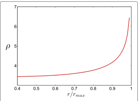
In practice,ρis a small constant. Considerα = 4 and
β =1. Figure 2 indicates the relationship betweenr/rmax
andρ. We see that whenr/rmax≤0.8,ρis smaller than 4.
We remark that in practice, there will be localization errors. They can be incorporated by requiring the mutual distance between nodes to be at least ρr + . Recall that is the maximum localization error. The incorpo-ration of localization error also increases the distance between hexagons (explained later) with the same color and thereby ensuring the transmissions from nodes in these hexagons are interference free.
Figure 2A plot ofρwhenα=4 andβ=1.
a number of methods; examples include [7,12] and [10]. Without loss of generality, in this paper, we will employ the following 3k2 coloring method when scheduling broad-cast. As we will see later, the color of a hexagon will be used to achieve interference-free transmissions in Section 4.2, where nodes located in hexagons with a different color are not allowed to transmit or receive simultaneously.
We are given a natural number k and a hexagonal tessellation with a hexagon radius of r/2, where r is the transmission range in GT. Define two vectors x = (3√3r/4, 3r/4)andy = (3√3r/4,−3r/4). These vectors have a length of 3r/2. Repeat the following process, see Algorithm 1, for allcolors; here,coloris an integer in the range [ 1, 3k2]; i.e., 1≤color ≤3k2. Start from an uncol-ored hexagon with centrehand then assign all hexagons with center ath+akx+bkywithcolor, wherea,b∈Z. For instance, supposek=2. We need to assign the same value
colorto all hexagons with centerh+3ax+3bywherea,b∈
Z. This process repeats until color=3k2=12. The result
Figure 3An example of hexagonal tessellation and coloring.
of 12 coloring is shown in Figure 3. Note,h+akx+bkyis a function ofaandb; both of which can be arbitrary inte-gers, e.g.,a = 1,b = −1, if there exists a hexagon in the network with centerh+akx+bky.
Algorithm 13k2-coloring method 1: input:r,k,xandy
2: output:3k2-colored hexagons 3: color←1
4: fori←1 to 2kdo 5: ifi≤kthen
6: forj←1 tok+i do
7: h←((2j−i−1)√3r/4,−(i−1)3r/4) 8: end for
9: else
10: forj←1 to 3k−i do
11: h←((2j+i−1−2k)√3r/4,−(i−1)3r/4) 12: end for
13: end if
14: Assigncolorto hexagons with centerh+akx+bky for alla,b∈Z,
15: color←color+1 16: end for
Lemma 1. (Huang et al. [7]). Algorithm 1 results in a3k2 coloring, and hexagons of the same color are separated by at least a distance of(3k−2)r/2.
According to Theorem 1 and Lemma 1, in order to apply Algorithm 1 under the SINR-based interference model, we need to set(3k−2)r/2 =ρr. In other words,
k= 2(ρ+2)/3 . Based on the transmission graphGT, a hexagon is said to becoveredby a nodev∈VT, if and only if nodev’s neighbors are in the said hexagon, excludingv. To distinguish nodes on the edges of hexagons, we assume each hexagon is left half open and right half close, with the topmost node included and the bottommost node excluded.
3.3 Problem formulation
Let(Bi,Ri,ti +kiT) denote the ith transmission, i,ki ∈ N, where eachBi(respectively,Ri) is the set of nodes that send (respectively, receive) the message at time slotti+ kiT, wheretiis the active time slot of nodes inRi. Given a wireless network with duty cycle and a source nodes∈V, the broadcast problem is to find a forwarding schedule,
B= {(B1,R1,t1+k1T),· · ·,(Bm,Rm,tm+kmT)}
SINR-based interference model, (iii)mi=1Ri= |V|and tm+kmT−(t1+k1T)is minimum. In other words, find an interference-free broadcast schedule that guarantees all nodes inVreceive the broadcast message interference-free in minimum time.
4 A distributed broadcast scheduler
We now present our distributed hexagon broadcast scheduling algorithm (HBA). We first describe HBA fol-lowed by our theoretical analysis confirming its O(1) -approximation ratio in terms of broadcast latency.
4.1 Broadcast structure
HBA starts by constructing a broadcast structure Tb before using the color of hexagons to derive a broad-cast schedule such that nodes located in hexagons with a different color are not allowed to transmit or receive simultaneously.
Firstly, we describe the construction of Tb; see Algorithm 2 for details. Each node first tessellates the net-work into equal hexagons with a radius ofr/2 and then gives a 3(2(ρ+2)/3 )2coloring to all hexagons (lines 5
and 6 in Algorithm 2). Note, as the radius of each hexagon isr/2, the maximum distance in each hexagon isr; that is, nodes located in the same hexagon are one-hop neighbors of each other.
Algorithm 2Broadcast structureTb
1: input:Transmission graphGT =(VT,ET(r)) 2: output:Tb=(Vb,Eb)
3: Vb← ∅,Eb← ∅ 4: foreach nodevinVT do
5: Tessellate the plane into equal hexagons with radius r/2, one of which is centered at(0, 0)
6: Apply Algorithm 1 to color all hexagons by setting k= 2(ρ+2)/3
7: H1(v)←u|ulies in the same hexagon asv∪{v}
8: H2(v)← {u|u∈N1(H1(v))andu∈/H1(v)} 9: Mark all hexagons asuncovered
10: whileH2(v)= ∅do
11: u ←a node inH1(v)covering mostuncovered
hexagons (break ties based on smaller ID) 12: foreachuncoveredhexagon covered byudo
13: w←a node with smallest ID among nodes in thisuncoveredhexagon andN1(u)
14: H2(v)←H2(v)\ {H1(w)∩H2(v)} 15: Eb←Eb∪ {(u,w)}
16: Mark thisuncoveredhexagon ascovered 17: end for
18: end while 19: end for
20: Vb←nodes inEb
Next, based on two-hop neighbors information, node
v places into set H1(v) neighbors that are in the same hexagon as itself and adds into set H2(v) nodes in the other hexagons that are the one-hop neighbors of nodes in H1(v) (lines 7 and 8 in Algorithm 2). Note that set H1(v)includes nodev. Since nodes inH1(v)are one-hop neighbors with each other and they are aware of two-hop neighbors information, nodes in the same hexagon will produce the sameH1andH2sets.
To reduce the number of transmissions, HBA selects a set of nodes from H1(v) that covers all neighbor-ing hexagons containneighbor-ing a neighbor; i.e., the selected nodes are neighbors of nodes inH2(v). Ideally, we want the chosen set to have a small cardinality. Specifically, HBA, applies line 9 to 18 in Algorithm 2 to produce the broadcast structure Tb = (Vb,Eb), where Vb contains nodes used to relay broadcast messages, i.e., providers
andreceptors, and Eb indicates the set of links between aproviderand its correspondingreceptor. Here,provider
is a node selected fromH1(v) and is used for relaying a broadcast message to its corresponding receptors; while areceptor is a node chosen from setH2(v) and is used to transmit a broadcast message to all other nodes in its hexagon.
Initially, HBA marks all hexagons as uncovered and then repeats the following iterations until H2(v) is empty. It first picks a node u ∈ H1(v) that covers the most uncovered hexagons (line 11 in Algorithm 2), and labels u as a provider. The next step is to select one corresponding receptor of u from each uncovered
hexagon. Specifically, for eachuncoveredhexagon, HBA will choose as the corresponding receptor a node w
with the smallest ID among nodes in N1(u); see line 13 in Algorithm 2. Then, it includes link (u,w) in the set Eb and removes nodes in H1(w) from H2(v), i.e., H2(v)\{H1(w)∩H2(v)} (lines 14 and 15 in Algorithm 2). It then marks the uncovered hexagon as covered. Note, provider u and its corresponding receptor w are located in different hexagons, and provider u (respec-tively, receptor w) has only one corresponding receptor
w (respectively, provider u) in the hexagon including w
(respectively,u).
After the execution of Algorithm 2, we have the broad-cast structureTb, whereVbcontains providers and recep-tors, and Eb indicates the link of a provider and its corresponding receptors.
We now use Figure 4 as an example to illustrate the operation of Algorithm 2. We only consider the broadcast structure of the hexagon with color 5. Recall that nodes in the same hexagon produce the same broadcast struc-tureTb. Hence, in the following description, we illustrate Algorithm 2 from the perspective of node v1. It starts
Figure 4HBA in operation.
{v1,v2,v3}andH2(v1)= {v4,v5,v6,v7,v8,v9,v10}. Nodev1
is first selected as the provider fromH1(v1)as it covers the mostuncoveredhexagons, i.e., hexagons with nodev4,
v5,v6, andv10. Next, nodev4,v5,v6, andv10are selected as the corresponding receptors of v1 and are removed
fromH2(v1), i.e.,H2(v1) = {v7,v8,v9}. Algorithm 2 then
marks the hexagons covered byv1ascoveredand adds into
the setEbthe links(v1,v4),(v1,v5),(v1,v6), and(v1,v10).
The other nodes in H1(v1), i.e.,v2 and v3, are handled
in a similar manner, and the final result is shown in Figure 4. For the hexagon with color 5, the set of providers is{v1,v2,v3}.
The aforementionedTbconstruction process yields the following property.
Lemma 2. For each hexagon H, there are at most 18 providers with corresponding receptors located inH.
Proof 1. Recall that a provider u and its corresponding receptor v are located in different hexagons and only one link(u,v) exists in Eb between these two hexagons. This means we only need to prove the number of hexagons cov-ered by receptors in a given hexagonHis upper-bounded by 18. As shown in Figure 3, for a given hexagon H with radius of r/2, it has at most 18 hexagons around it with a minimum distance less than r; that is, nodes inHcan cover at most 18 hexagons. Hence, this lemma holds.
4.2 Broadcast scheduling
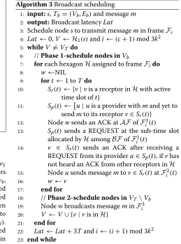
In this section, we describe the protocol used to broadcast a message from the source nodesto all other nodes inGT, see Algorithm 3.
Algorithm 3Broadcast scheduling 1: input:s,Tb=(Vb,Eb)and messagem 2: output:Broadcast latencyLat
3: Schedule nodesto transmit messagemin frameFc 4: Lat←0,V←H1(s)andi←(c+1)mod 3k2 5: whileV =VTdo
6: //Phase 1-schedule nodes inVb
7: foreach hexagonHassigned to frameFido 8: w←NIL
9: fort←1 toTdo
10: Sr(t)← {v|vis a receptor inHwith active time slot oft}
11: Sp(t)←u|uis a provider withmand yet to sendmto its receptorv∈Sr(t)}
12: Nodewsends an ACK atAFofFi1(t) 13: Sp(t)sends a REQUEST at the sub-time slot
allocated byHamongBFofFi1(t)
14: v ∈ Sr(t) sends an ACK after receiving a REQUEST from its provideru∈Sp(t), ifvhas not heard an ACK from other receptors inH 15: Nodeusends messagemtov∈Sr(t)atFi2(t) 16: w←v
17: end for
18: //Phase 2-schedule nodes inVT\Vb 19: Nodewbroadcasts messageminFi3 20: V ←V∪ {v|vis inH}
21: end for
22: Lat←Lat+3Tandi←(i+1)mod 3k2 23: end while
HBA schedules the transmission of nodes inGT in two phases. In phase 1, the algorithm only considers nodes inVb. Specifically, for each hexagon, denoted byH, HBA schedules the transmisison from a provideruto its cor-responding receptorvinH, where(u,v) ∈ Eb. In phase 2, HBA allows a receptor v in H to transmit a broad-cast message received in phase 1 to all other nodes inH. Furthermore, HBA schedules all tranmissions based on hexagons’ color, where those with a different color are not permitted to transmit or receive simultaneously.
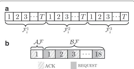
We divide time into different frames. A hexagon with the color value ofiis assigned to theith frame, denoted by Fi, where 1 ≤ i ≤ 3k2; recall that 3k2 is the num-ber of colors used by Algorithm 1. As shown in Figure 5a, each frameFi consists of three sub-frames, i.e.,Fi1,Fi2, andFi3, comprising of 3Ttime slots. For each hexagonH, the firstT time slot, i.e., sub-frameFi1, is used to deter-mine which providerufrom other hexagons is allowed to send a broadcast messagemto its corresponding receptor
a
b
Figure 5An illustration of frame and sub-frame structure.(a)An example of frameFi, and (b) An example of time slotFi1(t). Note, the sub-frame shown in(b)only applies to each slot ofF1
i(t).
all other nodes inH. Specifically, phase 1 is conducted in F1
i andFi2, and phase 2 is carried out inFi3.
Letcbe the color of the hexagon containing source node
s. Therefore, node sinitiates the broadcast by transmit-ting a messagemto all nodes in its hexagon in frameFc. After that, HBA, see Algorithm 3, starts from frameFi, whereiis initially set to(c+1)mod 3k2; that is, it starts from the next frame ofFc(line 4 in Algorithm 3). Then, HBA repeats the following iterations until all nodes in the network receive the broadcast message.
In phase 1, for each hexagonHassigned to frameFi, i.e., they have colori, letSr(t)denote the set of receptors inHwith active time slott, andSp(t)denotes the set of providers that have received broadcast messagembefore but have yet to sendmto their corresponding receptors in
Sr(t)(lines 10 and 11 in Algorithm 3), where 1 ≤ t≤ T. Recall that these providers will have to wake up at timetto communicate with the receptors inSr(t). LetFi1(t)be the time slottof sub-frameFi1, where 1≤t≤T. Denote by
wa receptor inHthat received a REQUEST message from its corresponding provider beforeFi1(t), andwis initially set to null. For any receptorv∈Sr(t),vfirst listens to the channel for an ACK message from a receptorwwhen it wakes up at time slotFi1(t)(line 12 in Algorithm 3). This ACK is sent in theAF slot; see Figure 5b. Then, for any provideru∈Sp(t), it will send a REQUEST message to its receptorv∈Sr(t)asking it to receive a broadcast message in sub-frameFi2(line 13 in Algorithm 3).
When receptorvreceives the REQUEST message from provideru, ifvhas not received any ACK message from other receptors inH, nodevreplies with an ACK mes-sage tou. Otherwise, it does not respond to REQUEST messages (line 14 in Algorithm 3). As shown in line 16 of Algorithm 3, the selected receptorvis assigned tow, and it is responsible for sending an ACK message in subsequent AF slots inFi1(t)(line 12 in Algorithm 3). This ensures all nodes waking up in subsequent slots are aware that aw
node is available and thus stop responding to REQUEST messages.
We now discuss how providers in Sp(t) transmit their REQUEST message in an interference-free manner. For each time slot in Fi1(t), we further divide it into two parts,AF andBF; see Figure 5b. As mentioned earlier, AF is used by receptors in Sr(t) to listen to the chan-nel for an ACK message and for node w, if present, to transmit an ACK. The second part, namelyBF, is divided into 18 sub-time slots, which is equal to the number of hexagons aroundH that have a minimum distance less thanr; cf. Lemma 2. We allocate these 18 sub-time slots to these neighboring hexagons according to their ID or color. Hence, a provideru ∈ Sp(t) is only able to send a REQUEST message to its corresponding receptor v ∈ Sr(t) in the sub-time slot corresponding to its hexagon. A receptorvis then required to reply with an ACK mes-sage in the same sub-time slot. As shown in Figure 5b, we assume each sub-time slot is sufficient to receive a REQUEST message and transmit an ACK message for receptorv.
During time slottof sub-frameFi2, denoted byFi2(t), where 1 ≤ t ≤ T, the broadcast messagemis transmit-ted from the provideruto receptorvwith active time slot
t (line 15 in Algorithm 3). Note, only one provider uis selected inFi1to relay the broadcast message in sub-frame F2
i to hexagonH.
In phase 2, after receiving the broadcast message m, receptor vwill broadcast message m to all other nodes in the same hexagon as v, i.e., H, in sub-frame Fi3. The broadcast is carried out when these nodes wake up (line 19 in Algorithm 3). Finally, HBA updatesito(i+1)mod 3k2
and repeats the above steps until all nodes receive the broadcast messagem.
We now illustrate the operation of Algorithm 3 using Figure 4. Consider the hexagon with color 8. Assume receptors v6, v11, andv12 have the same active time slot oft, and their corresponding providers,v1, v13, andv14, have received a broadcast messagem, which it has yet to send to v6, v11, andv12. Hence, as per Algorithm 3, we getSr(t) = {v6,v11,v12}andSp(t) = {v1,v13,v14}. Nodes
inSr(t), which are in hexagon 8, execute Algorithm 3 in frame F8. In the AF sub-time slot of F81(t), receptors
inSr(t)listen to the channel for an ACK message. Sup-pose that no ACK message is sent at AF by a nodew. Also, in this case, we assume that the transmitting order of providers isv1,v13, andv14. As mentioned, the sub-time
slots inBFcan be assigned as per hexagon ID or color. In this example, providerv1first sends a REQUEST tov6. On
receiving this REQUEST,v6replies with an ACK
imme-diately. After receiving this ACK from v6, provider v1
providerv1 sendsmtov6. In sub-frameF83, receptorv6
broadcastsmto nodesv11andv12.
4.3 Distance-based backoff
Recall that the BF portion of Fi1(t) is divided into 18 sub-time slots. A possible optimization to shortenBF is by employing a distance-based backoff method. When a provider wants to send a REQUEST message, it first backs off for a period of time. This backoff duration depends on the distance between the provider and the hexagon containing its corresponding receptor. The smaller the distance, the shorter the backoff duration. Specifically, assume that a network operator decides to reduce the BFduration toTbackoff. This so calledbackoff time bound
can be divided intoW ≤ 18 sub-time slots. Note, each sub-time slot is sufficient for transmitting an ACK and receiving a REQUEST message. Let d be the distance between a provideruand the centre of hexagonH con-tainingu’s receptor. We getd ≥ √3r/4 becauseuis not included inH, and the distance betweenH’s edge andH’s centre is√3r/4. Denote byqthe ratio between√3r/4 and
d, i.e.,q=
√
3r
4d , whereq≤1. For provideru, it computes its backoff durationtbackoffusing the following equation,
tbackoff=
W(1−q)Tbackoff
W +X (2)
whereXis random period of the time generated from the range−Tbackoff valueXreduces the chance of interference when two or more providers have the sameq.
5 Analysis
The following set of theorems assert the correctness and approximation ratio of HBA in terms of broadcast latency and transmission times.
Theorem 2. HBA yields a correct and interference-free broadcast schedule.
Proof 2. According to Theorem 1, transmissions are inter-ference free as long as the mutual distance between trans-mitters or receivers is larger thanρr. Hence, we only need to prove that simultaneous transmissions carried out by HBA are separated byρr.
Recall that in GT, by design, the mutual distance between hexagons sharing the same color is larger thanρr. For each frameFi, only nodes in hexagons with the same color of i are scheduled by HBA. Considering sub-frames
F2
i andFi3, only providers and their corresponding recep-tors are allowed to send a broadcast message to nodes in hexagons with the same color of i. These receptors lie in hexagons with color value of i, and hence, their mutual
distance is larger thanρr. Thus, these simultaneous trans-missions during sub-frames Fi2 and Fi3 are interference free by Theorem 1.
Then, we prove the transmissions in sub-frameFi1are also interference free. Only providers and their correspond-ing receptors are allowed to send a REQUEST and ACK duringFi1. For hexagonHwith color value of i, the trans-missions of providers and their receptors inHare assigned with non-overlapping sub-time slots in Fi1, and hence, transmissions in the same hexagonHare interference free. For different hexagons which share the same color of i, the mutual distance of receptors lying in them is lower-bounded by ρr. According to Theorem 1, simultaneous transmissions in different hexagons during sub-frameFi1 are also interference free.
Theorem 3. HBA produces a constant approximation for the MLBS problem with a ratio of 92(ρ+2)/3 2T in terms of broadcast latency.
Proof 3. The theoretical lower-bound of the MLBS prob-lem is R, i.e., the radius of the network with respect to the source node s. To compare the broadcast latency of HBA algorithm with the theoretical lower-bound R, we consider the BFS tree of the transmission graph GTrooted at s. This tree divides the network into layers L1,L2,· · ·,LR. Let ti denote the maximum reception time of nodes in Li, where 1 ≤ i ≤ R. Then, we prove for each layer Li, we have ti≤ti−1+92(ρ+2)/3 2T. We prove this by induction.
L1only contains source node s, and thus t1 = 0. Nodes in L2are the one-hop neighbors of s. Thus, for L2, it holds true because it takes a frame, i.e.,3T, for node s to broad-cast the message m to L2, i.e., t2 = t1 +3T. Then, we also prove this is true for layer i, where 3 ≤ i ≤ R. Recall that nodes in Liare the one-hop neighbors of Li−1. After ti−1, receptors in Liwill take at most32(ρ+2)/3 2 frames to get the message m from providers in Li−1 and broadcast m to other nodes in Li, where32(ρ+2)/3 2 is the maximum color number used by Algorithm 1. Note, a frame contains3T time slots. Thus, for each layer Li, ti≤ti−1+92(ρ+2)/3 2T. After(R−1)32(ρ+2)/3 2 frames, nodes in LRwill receive the broadcast message m. Hence, the broadcast latency of HBA is upper-bounded by (R−1)92(ρ+2)/3 2T <92(ρ+2)/3 2TR.
Theorem 4. The number of REQUEST, ACK, and broad-cast messages in HBA is upper-bounded by18NH, TNH, and(T +1)NH respectively, where NH is the number of hexagons required to cover the entire network.
REQUEST message is only sent once from a provider to its corresponding receptor. It means, for each hexagonH, its receptors receive at most 18 REQUEST messages. Hence, given NH hexagons, the number of REQUEST messages is upper-bounded by 18NH. Next, we show that the num-ber of ACK messages is upper-bounded by TNH. For each hexagonH, the ACK message is first sent by a receptor v inHin response to a REQUEST message from v’s corre-sponding provider. An ACK message is sent once in each time slot until sub-frameFi1ends. SinceFi1consists of T time slot, the maximum transmission time of ACK is T for each hexagon. To sum up, the maximum number of ACK sent during the broadcast is TNH. Last, we show the maxi-mum number of broadcast messages transmitted by HBA is (T+1)NH. As illustrated in Section 4.2, during sub-frame F2
i for a hexagonH, only one provider is allowed to trans-mit a broadcast message to its corresponding receptor v in
H. During each time slot ofFi3, receptor v will transmit a broadcast message at most T times to its neighbors inH. The maximum number of broadcast messages transmitted in a hexagon is thus T+1, meaning the total number of broadcast messages is upper-bounded by(T+1)NH.
6 Evaluation
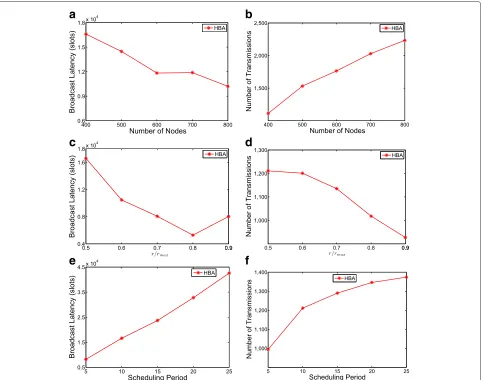
In this section, we outline the research methodology used to evaluate the performance of HBA. In our experiments, we measure each algorithm against two metrics: broad-cast latencyandnumber of transmissions. In our experi-ments, we fix α = 4,β = 1 and rmax = 100 m. We place wireless nodes in a square area of 700×700 m2 ran-domly, while changing the number of nodes, transmission ranger, and scheduling periodT. In addition, we ensure that the resulting WSN is connected. For each experiment, we change one network configuration while the other two remain unchanged. Each experiment is conducted on 50 randomly generated topologies. Moreover, for each topol-ogy, we run the algorithms ten times; for each run, we select a source node uniformly and randomly. Hence, each result is an average of 50×10 simulation runs.
6.1 Performance of HBA
In Figure 6a,b, we delineate the broadcast latency and number of transmissions for different number of nodes, respectively. The value of r is fixed at 50 m, and T
is set to 10. As shown in Figure 6a, we see that the broadcast latency of HBA decreases as the number of nodes increases. The reason is as follows. For a fixed area, the network becomes denser when the number of nodes becomes larger. As a result, when the network becomes denser, there are more links and path lengths become shorter. However, we observe that the number of transmissions increases with higher number of nodes in Figure 6b. The reason is that more hexagons will be filled with nodes when the number of nodes becomes larger,
and hence, more transmissions are required to propagate the broadcast message to these hexagons.
Figure 6c,d shows the performance of HBA under dif-ferent r/rmax, where ris the transmission range in GT, andrmaxis the maximum transmission range with a fixed
value of 100 m. In this experiment, the number of nodes is fixed to 400,T is set to 10, andrranges from 50 to 90 m. As shown in Figure 6c, the broadcast latency decreases whenrranges from 50 to 80 m. This is because a larger transmission rangerleads to more links and higher con-nectivity. As a result, HBA is able to find shorter broadcast paths. On the other hand, according to Theorem 1, a larger
ralso prevents more nodes from transmitting simultane-ously, which will result in longer broadcast paths. Hence, when the transmission rangerexceeds 80 m in Figure 6c, the broadcast latency starts to increase. We see that in Figure 6d the number of transmissions decreases with increasingr. This is because the number of hexagons used to cover the network becomes smaller when rbecomes larger. Hence, there are fewer transmissions when r is large.
Figure 6e,f depicts the performance of HBA for differ-ent scheduling periodsT. The value ofT ranges from 5 to 25 (r = 50 m and the number of nodes is set to 400). Note that the broadcast latency and number of transmis-sions increase with higherT values. A largerT will result in larger frames and thereby leads to higher broadcast latency. Consequently, for each hexagon, a receptor needs to transmit more times to its neighbors with different active time slots.
6.2 Performance of HBA versus tree-based algorithm
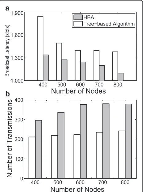
In this section, we compare HBA against the tree-based algorithm [7] for always-on networks. Recall that the tree-based algorithm [7] is the first centralized method designed for always-on networks under SINR-based inter-ference model. In this respect, we note that HBA is the first distributed algorithm designed for duty-cycle net-works under the SINR-based interference model. In order to compare HBA faithfully against the tree-based algo-rithm [7], the scheduling period used by HBA is set to 1, i.e.,T = 1, meaning HBA also works in the always-on mode.
a
b
c
d
e
f
Figure 6Performance of HBA under different network configurations.The impact on broadcast latency and number of transmissions given varying number of nodes, see(a, b), different r/rmaxvalues, see(c, d), and scheduling period, see(e, f).
nodes using HBA is about 50% more than that of the tree-based algorithm. This is because the tree-tree-based algorithm determines the transmitting nodes in the maximum inde-pendent set centrally. This, however, does not consider the cost of requiring all nodes to synchronize their wake-up schedule and collating such information centrally.
7 Conclusions
In this paper, we have studied the minimum latency broadcast scheduling problem in duty-cycled WSNs. To achieve interference-free broadcast, we designed a novel algorithm, called HBA, for nodes that employ a ran-dom duty-cycle schedule. We prove that HBA provides a correct and interference-free schedule, produces a low broadcast latency, and has low overheads. Our simulation results show HBA to have better performance in terms of broadcast latency than the tree-based algorithm [7]. As a future work, we are currently looking into implementing
HBA in the more realistic and probabilistic interference model where a message can be received successfully with varying probability as per SINR levels.
Endnote
aAρ-approximation algorithm, withapproximation
ratioρ >1, if given a problem instanceIto minimize and with optimal solutionOPT(I), produces a solution that is bounded byρ·OPT(I).
Appendix
Lemma 3. Given a set L of links, if the mutual distance of senders in L are greater thanρr, set L is independent,
whereρ=1+1−(r/8rβ
max)α
2
α−2+ α−11+3
1/α
.
a
b
Figure 7Performance of HBA versus tree-based algorithm in terms of broadcast latency (a) and number of transmissions (b) over varying number of nodes.
concentric rings ringk with widthρr. Ring ringk contains all senders w of links in L satisfying kρr ≤ d(w,u) < (k+1)ρr. The first ring ring0only contains sender u. We now consider all senders w∈ringkfor some integer k>0.
First, we consider the distance between any senders w in ringk and u. As per the construction of rings, we have d(w,u) ≥ kρr for ring ringk. Note that, d(u,v) ≤ r and ρ >1. Applying the triangle inequality, the lower-bound of d(w,v)for ringkis,
d(w,v)≥d(w,u)−d(u,v) ≥kρr−r
> (ρ−1)kr
(3)
Next, observe that for any senders w in ringk, the disk centered at w with a radius of12ρr is non-overlapping with other senders in ringk, and such a disk is fully contained in an extended ring of ringk, with an extra width of 12ρr at each side of ringk. Then, by referring to the ratio between the area of this extended ring and the disk with a radius
of 12ρr, the number of senders contained in ringkis upper-bounded by8(2k+1)as per Equation 4.
π(k+3/2)2(ρr)2−π(k−1/2)2(ρr)2
π(1/2ρr)2 =8(2k+1)
(4)
The total interference Ik emanating from ringk is bounded by
Ik=
w∈ringkPd(w,v)
−α
≤8(2k+1)P((ρ−1)kr)−α
(5)
Summing up the total interferences I over all rings yields
I=∞k=1Ik
=∞k=18(2k+1)P((ρ−1)kr)−α
(6)
Recall that d(u,v)≤r and N =P/βrαmax, where rmaxis the maximum transmission range in the absence of inter-ference. If v successfully receives a message from u if and only if the following condition holds:
SINR= Pd(u,v)
−α
I+N
≤ ∞ Pr−α
k=18(2k+1)P((ρ−1)kr)−α+P/βrαmax
= ∞ β
k=18β(2k+1)(ρ−1)−αk−α+(r/rmax)α
≤β
(7)
According to inequality 7, such SINR is at leastβif and only if
∞
k=18β(2k+1)(ρ−1)
−αk−α+(r/r
max)α ≤1 (8)
According to Riemann zeta function, we know that
∞
k=1k−α ≤α−11+1, whereα >2. Plugging this in, we have
∞
k=18(2k+1)k
−α ≤8 2
α−2 + 1
α−1+3
(9)
According to inequality 8 and 9, we have
∞
k=18β(2k+1)(ρ−1)
−αk−α+(r/r
max)α
=8β
2
α−2+ 1
α−1+3
(ρ−1)−α+(r/rmax)α
≤1
(10)
When ρ = 1 + 1−(r/8rβ
max)α
2
α−2+α−11+3
1/α
receive the message successfully in L. In conclusion, set L is independent.
Lemma 4. Given a set L of links, if the mutual distance of receivers in L is greater thanρr, set L is independent, where ρ=1+ as receiver v, we then divide the receivers in L into con-centric rings ringk. Recall that the length of each link is upper-bounded by r in L. For a sender w whose receivers lie in ringk, d(w,v)is lower-bounded byρkr−r≥(ρ−1)kr. That is, for ringk, the distance between interfered sender w and receiver v is no smaller than(ρ−1)kr. Next, using
the same argument as Lemma 5, we conclude that L is also independent.
Theorem 5. Given a set L of links, in order for set L to be independent, it is sufficient to have:
1. The mutual distance of senders are all greater than ρr; OR
2. The mutual distance of receivers are all greater than ρr.
Proof 7. This is proved by Lemma 5 and 6.
Competing interests
The authors declare that they have no competing interests.
Acknowledgements
This project is supported by the CSC-UoW joint scholarship program.
Received: 2 October 2014 Accepted: 12 February 2015
References
1. C Perkins, E Royer, inIEEE WMCSA. Ad-hoc on-demand distance vector routing (New Orleans, LA, USA, 1999)
2. W Nan, S Xue-li, inIEEE IITAW. Research on nodes location technology in wireless sensor networkunderground (Nanchang, China, 2009) 3. S Brown, C Sreenan, Updating software in wireless sensor networks: A
survey (2006). Technical Report UCC-CS-2006-13-07, University College Cork, Ireland, (2006)
4. R Gandhi, Y-A Kim, S Lee, J Ryu, P-J Wan, inIEEE INFOCOM. Approximation algorithms for data broadcast in wireless networks (Rio de Janeiro, Brazil, 2009)
5. R Gandhi, A Mishra, S Parthasarathy, Minimizing broadcast latency and redundancy in ad hoc networks. IEEE/ACM Trans. Netw.16(4), 840–851 (2008)
6. Z Chen, C Qiao, J Xu, T Taekkyeun Lee, inIEEE INFOCOM. A constant approximation algorithm for interference aware broadcast in wireless networks (Anchorage, Alaska, USA, 2007)
7. S-H Huang, P-J Wan, J Deng, Y Han, Broadcast scheduling in interference environment. IEEE Trans. Mobile Comput.7(11), 1338–1348 (2008) 8. S-H Huang, P-J Wan, X Jia, H Du, W Shang, inIEEE INFOCOM.
Minimum-latency broadcast scheduling in wireless ad hoc networks (Anchorage, AK, USA, 2007)
9. R Mahjourian, F Chen, R Tiwari, M Thai, H Zhai, Y Fang, inProceedings of the 9th ACM international symposium on Mobile ad hoc networking and
computing,MobiHoc ’08. An approximation algorithm for conflict-aware broadcast scheduling in wireless ad hoc networks (ACM New York, NY, USA, 2008), pp. 331–340
10. R Tiwari, T Dinh, M Thai, On centralized and localized approximation algorithms for interference-aware broadcast scheduling. IEEE Trans. Mobile Comput.12, 233–247 (2013)
11. P Gupta, P Kumar, The capacity of wireless networks. IEEE Trans. Inf. Theory.46(2), 388–404 (2000)
12. S Huang, S-Y Chang, H-C Wu, P-J Wan, Analysis and design of a novel randomized broadcast algorithm for scalable wireless networks in the interference channels. IEEE Trans. Wireless Commun.9(7), 2206–2215 (2010)
13. P-J Wan, L Wang, O Frieder, inIEEE MASS. Fast group communications in multihop wireless networks subject to physical interference (Macau SAR, China, 2009)
14. W Ye, J Heidemann, D Estrin, inIEEE INFOCOM. An energy-efficient MAC protocol for wireless sensor networks (New York, NY, USA, 2002) 15. K-W Chin, Pairwise: A novel time hopping MAC for wireless sensor
networks. IEEE Trans. Consumer Electron.55(4), 288–304 (2000) 16. H Lim, C Kim, Flooding in wireless ad hoc networks. Comput. Commun.
24(3), 353–363 (2001)
17. S Ni, YCYC Tseng, J Sheu, inACM MOBICOM. The broadcast storm problem in a mobile ad hoc network (Seattle, WA, USA, 1999)
18. F Ferrari, M Zimmerling, L Thiele, O Saukh, inIPSN. Efficient network flooding and time synchronization with glossy (Chicago, IL, USA, 2011) 19. Y Sasson, D Cavin, A Schiper, inIEEE WCNC. Probabilistic broadcast for
flooding in wireless mobile ad hoc networks (New Orleans, LA, USA, 2003) 20. F Stann, J Heidemann, R Shroff, MZ Murtaza, inACM SenSys. Rbp: robust
broadcast propagation in wireless networks (Boulder, CO, USA, 2006) 21. J Hong, J Cao, W Li, S Lu, D Chen, inIEEE ICC. Sleeping schedule-aware
minimum latency broadcast in wireless ad hoc networks (Dresden, Germany, 2009)
22. X Jiao, W Lou, J Ma, J Cao, X Wang, X Zhou, Minimum latency broadcast scheduling in duty-cycled multi-hop wireless networks. IEEE TPDS.
23(1), 110–117 (2012)
23. X Xu, J Cao, P-J Wan, inWASA. Fast group communication scheduling in duty-cycled multihop wireless sensor networks (Fusionopolis, Singapore, 2012)
24. P Gupta, PR Kumar, The capacity of wireless networks. IEEE Trans. Inf. Theory.46(2), 388–404 (2000)
25. Y Gu, T He, inIEEE ICDCS. Bounding communication delay in energy harvesting sensor networks (Genoa, Italy, 2010)
26. M Maróti, B Kusy, G Simon, A Lédeczi, inSenSys. The flooding time synchronization protocol (Baltimore, Maryland, 2004)
27. Y Gu, T He, inACM SenSys. Data forwarding in extremely low duty-cycle sensor networks with unreliable communication links (ACM, Sydney, Australia, 2007)
28. P Dutta, D Culler, inSenSys. Practical asynchronous neighbor discovery and rendezvous for mobile sensing applications (ACM Raleigh, NC, USA, 2008)
29. J Hong, W Li, S Lu, J Cao, D Chen, inIEEE ICPADS. Sleeping schedule aware minimum transmission broadcast in wireless ad hoc networks
(Melbourne, Victoria, Australia, 2008)
30. C Hua, T-SP Yum, Asynchronous random sleeping for sensor networks. ACM Trans. Sensor Netw.3(3) (2007)
31. G Han, H Xu, TQ Duong, J Jiang, T Hara, Localization algorithms of wireless sensor networks: A survey. Springer Telecommunication Syst.
52(4), 2419–2436 (2013)
32. O Goussevskaia, T Moscibroda, R Wattenhofer, inACM POMC. Local broadcasting in the physical interference model (ACM, Toronto, Canada, 2008)
33. MM Halldórsson, P Mitra, inACM FOMC. Towards tight bounds for local broadcasting (ACM, Madeira, Portugal, 2012)