R E S E A R C H
Open Access
Systematic construction, verification and
implementation methodology for LDPC codes
Hui Yu
*, Jing Cui, Yixiang Wang and Yibin Yang
Abstract
In this article, a novel and systematic Low-density parity-check (LDPC) code construction, verification and
implementation methodology is proposed. The methodology is composed by the simulated annealing based LDPC code constructor, the GPU based high-speed code selector, the ant colony optimization based pipeline scheduler and the FPGA-based hardware implementer. Compared to the traditional ways, this methodology enables us to construct both decoding-performance-aware and hardware-efficiency-aware LDPC codes in a short time. Simulation results show that the generated codes have much less cycles (length 6 cycles eliminated) and memory conflicts (75% reduction on idle clocks), while having no BER performance loss compared to WiMAX codes. Additionally, the simulation speeds up by 490 times under float precision against CPU and a net throughput 24.5 Mbps is achieved. Finally, a net throughput 1.2 Gbps (bit-throughput 2.4 Gbps) multi-mode LDPC decoder is implemented on FPGA, with completely on-the-fly configurations and less than 0.2 dB BER performance loss.
Keywords:low-density parity-check codes, simulated annealing, ant colony optimization, graphic processing unit, decoder architecture
1. Introduction
Low-density parity-check (LDPC) code is first proposed by Gallager [1] and rediscovered by Mackay and Neal since they introduce Tanner Graph [2] into LDPC code [3]. LDPC code with soft decoding algorithms on Tanner Graph can achieve outstanding capacity and approach Shannon limit over noisy channels at moderate decoding complexity [4]. Most algorithms root from the famous believe propagation (BP) algorithm, such as min-sum algorithm (MSA) with simplified calculation, modified MSA (MMSA) [5] with improved BER performance and layered versions [6] with fast decoding convergence.
The existence of“cycle”in Tanner Graph is a critical constraint of the above algorithms, as it breaks the
“message independence hypothesis” and degrades the BER performance. As a result,“girth”becomes an impor-tance metric of estimating the performance of the LDPC code. The progressive edge-growth (PEG) algorithm [7] is a girth-aware construction method that tries to make shortest cycle as large as possible. Approximate cycle extrinsic (ACE) message degree constraint is further
combined into PEG [8] to lower error floor. However, these performance-aware methods do not take hardware implementation into account, which usually result in low efficiency or high complexity.
As to the decoder implementation, the fully-parallel architecture [9] is first proposed for achieving the highest decoding throughput, but the hardware complexity due to the routing overhead is very high. The semi-parallel layered decoder [10] is then proposed to achieve the trade-off between hardware complexity and decoding through-put. Memory conflict is a critical problem for layered decoder, which is modeled as a single-layer traveling sales-man problem (TSP) in [11]. However, this model ignores
“element permutation”, i.e., the order assignment of the edges in each layer, and its search does not cover the entire solution space. Further, fully-parallel graphic processing unit (GPU) based implementation is also proposed in [12].
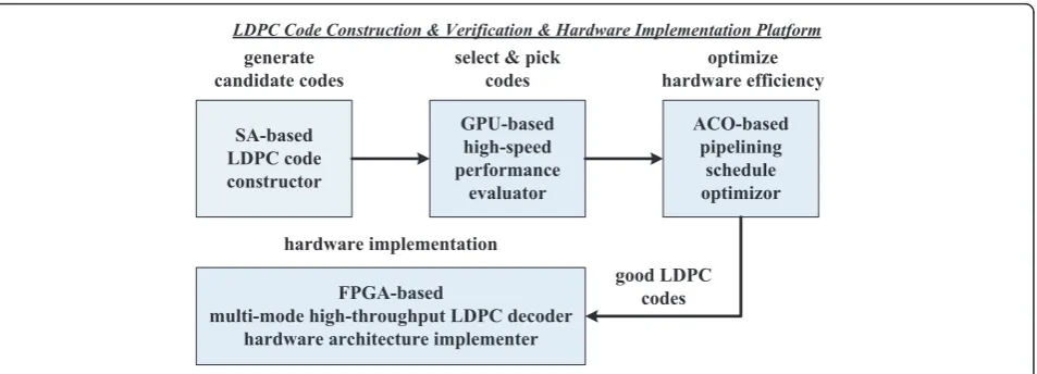
In this article, a novel and systematic LDPC code con-struction, verification, and implementation methodology is proposed, and a software and hardware platform is implemented, which is composed by four modules as shown in Figure 1. The simulated annealing (SA) based LDPC code constructor continuously constructs good candidate codes. The BER performance of the generated * Correspondence: [email protected]
Department of Electronic Engineering, Shanghai Jiao Tong University, Shanghai, P. R. China
codes, especially the error floor, is then evaluated by the high-speed GPU based simulation platform. Next, the hardware pipeline of the selected codes are optimized by the ant colony optimization (ACO) based scheduling algorithm, which can reduce much of the memory con-flicts. Finally, detailed implementation schemes are pro-posed, i.e.,reconfigurable switch network(adopted by [13]), offset-threshold decoding,split-row MMSA core, early-stop-ing schemeandmulti-block scheme, and the corresponding multi-mode high-throughput decoder of the optimized codes is implemented on FPGA. The novelties of the pro-posed methodology are listed as follows:
•Compared to traditional methods (PEG, ACE), the SA-based constructor takes both decoding perfor-mance and hardware efficiency into consideration dur-ing construction process.
•Compared to existed work [11], the ACO-based sche-duler covers both layer and element permutation, and maps the problem to a double-layer TSP, which is a complete solution and can provide better pipelining schedule.
•Compared to existed works, the GPU-based evaluator first implements the semi-parallel layered architecture on GPU. The obtained net throughput is similar to the highest report [12] (about 25 Mbps), while the pro-posed scheme has higher precision and better BER per-formance. Further, we put the whole coding and decoding system into GPU rather than a single decoder.
•Compared to existed FPGA or ASIC implementa-tions [14-16], the proposed multi-mode high-through-put decoder not only supports multiple modes with completely on-the-fly configurations, but also has a performance loss within 0.2 dB against float precision and 20 iterations, and a stablenet-throughput721.58 Mbps under code rate 1/2 and 20 iterations. With
early-stopping scheme, anet-throughput1.2 Gbps is further achieved on Stratix III FPGA.
The remainder of this paper is organized as follows. Section 2 presents the background of our research. Sections 3, 4, and 5 introduces the ACO based pipeline scheduler, the SA based code constructor and the GPU based performance evaluator, respectively, followed by hardware implementation schemes and issues of the multi-mode high-throughput LDPC decoder discussed in Section 6. Simulation results are provided in Section 7 and hardware implementation results are given in Section 8. Finally, Section 9 concludes this article.
2. Background
2.1. LDPC codes and Tanner graph
An LDPC code is a special linear block code, character-ized by a sparse parity-check matrix Hwith dimensions M ×N; Hj,i=1 if code bit iis involved in parity-check equationj, and 0 otherwise. An LDPC code is usually described by its Tanner Graph, a bipartite graph defined on the code bit set ℝand parity-check equation set ℂ, whose elements are called a “bit node” and a “check node”, respectively. An edge is assigned between bit nodeBNiand check nodeCNjif Hj,i= 1. A simple 4 × 6 LDPC code and the corresponding Tanner Graph is shown in Figure 2.
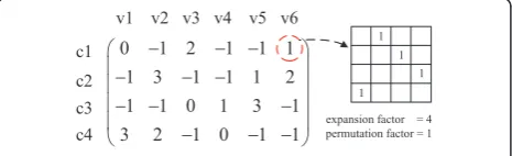
Quasi-cyclic LDPC codes (QC-LDPC) is a popular class of structured LDPC codes, which is defined by its base matrixHb, whose elements satisfying−1≤Hjb,i<zf.zf is called the expansion factor. Each element in the base matrix should be further expanded to azf×zfmatrix to obtainH. The elementsHbj,i=−1 are expanded to zero
matrices, while L(Qi) =L(ci) +
j∈ci
L(rji) =L(qij) +L(rji) 6$EDVHG
/'3& FRGH FRQVWUXFWRU
*38EDVHG KLJKVSHHG SHUIRUPDQFH
HYDOXDWRU
$&2EDVHG SLSHOLQLQJ
VFKHGXOH RSWLPL]RU JHQHUDWH
FDQGLGDWH FRGHV
VHOHFW SLFN FRGHV
RSWLPL]H KDUGZDUH HIILFLHQF\
JRRG /'3& FRGHV
/'3& &RGH &RQVWUXFWLRQ 9HULILFDWLRQ +DUGZDUH ,PSOHPHQWDWLRQ 3ODWIRUP
)3*$EDVHG
PXOWLPRGH KLJKWKURXJKSXW /'3& GHFRGHU KDUGZDUH DUFKLWHFWXUH LPSOHPHQWHU
KDUGZDUH LPSOHPHQWDWLRQ
are expanded to a cyclic-shift identity matrices with per-mutation factors Hbj,i≥0. QC-LDPC is naturally avail-able for layered algorithms, whose j-th row is exactly layerj. We call the“1"s of j-th row as the set p=Hbj,i. See Figure 3 for an example of a 4 × 6 base matrix with zf= 4.
2.2. The BP algorithm and effect of cycle
The BP algorithm is a general soft decoding scheme for codes described by Tanner Graph. It can be viewed as the process of iterative message exchange between bit nodes and check nodes. For each iteration, each bit node or check node collects the messages passed from its neighborhood, updates its own message and passes the updated message back to its neighborhood. BP algo-rithm has many modified versions, such as log-domain BP, MSA, and layered BP. All of them originate from the basic log-domain message passing equations, given as follows.
whereL(ci) is the initial channel message,L(qij) is the message passing fromBNi toCNj,L(rji) is the message of inverse direction, and L(Qi) is the a-posteriori of bit node BNi. Ci is the neighbor set of BNi, ℛj is the
neighbor set ofCNj. (x) = loge x+ 1
ex−1. These equations can also be applied in layered BP, the difference is that theL(qij) andL(rji) should be updated in each layer of the iteration.
The above equations requires the independence of all the messages L( qi′j), i′ Î ℛj and Hbj,k. However, the existence of “cycle” in Tanner Graph invalidates this independence assumption, thus degrades the BER per-formance of BP algorithm. A length 6 cycle is shown with bold lines in Figure 2. In this case, if BP algorithm proceeds for more than three iterations, the receive messages of the involved bit nodes v2,v4,v5 will partly contain its own message sent three iterations before. For this reason, the minimum cycle length in the Tanner Graph, called“girth”, has a strong relationship with its BER performance, and is considered as an important metric in LDPC code construction algorithms (PEG, ACE) [7,8].
2.3. Decoder architecture and memory conflict
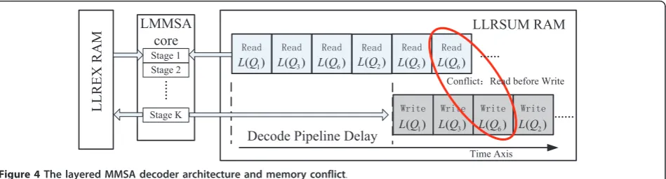
The semi-parallel structure with layered MMSA core is a popular decoder architecture due to its good tradeoff among low complexity, high BER performance and high throughput. As shown in Figure 4, the main compo-nents in the top-level architecture include an LLRSUM RAM storingL(Qi), an LLREX RAM storing L(rji) and a layered MMSA core pipeline. The two RAMs should be readable and writable. Old values ofL(Qi) andL(rji) are read, and new values are calculated through the pipeline and written back to RAMs. For QC-LDPC codes, the values are processed layer by layer, and the“1"s in each layer is processed one by one.
Memory conflict is a critical problem that constrains the throughput of the semi-parallel decoder. Essentially, memory conflict occurs when the read-after-write (RAW) dependency of L(Qi) is violated. Note that the new value of L(Qi) will not be written back to RAM until the pipelined calculation finishes. If L(Qi) is again needed during this calculation period, the old value will be read, while the new one is still under processing, see L(Q6) in Figure 4. This case happens when the layersj and j + l have “1"s in the same position
i(Hbj,i≥0,Hbj+l,i≥0). We call it a gap-lconflict. Memory conflict slows the decoding convergence and thus reduces the BER performance. The traditional method of handling memory conflict is to insert idle clocks in the pipeline, with the cost of throughput reduction. It’s obvious that the smallerl, the more idle clocks should be inserted, since the pipeline need to wait at least K stages before writing back the new values. Usually, the number of gap-1, gap-2, gap-3
Y Y Y Y Y Y
WKH SRVLWLRQ RI VSOLW URZ
Figure 2H matrix and Tanner Graph of LDPC.
SHUPXWDWLRQ IDFWRU
conflicts, denote c1, c2 and c3, are considered as the metrics of measuring memory conflict.
3. The ACO-based pipelining scheduler
In this section, we propose the ACO-based pipeline scheduling algorithm to minimize memory conflict. We first formulate this problem, then map it to the double-layered TSP and finally use ACO to solve it.
3.1. Problem formulation
Consider a QC LDPC code described by its base matrix Hwith dimensions M ×N. Thus, there are M layers. Denotewm,1≤m≤M as the number of elements ("1"s) in m-th layer. Denote hm,n, 1 ≤ n≤ wm as the column index inHof then-th element,m-th layer. Additionally, we assume the core pipeline isKstages.
As discussed above, the decoder processes all the“1"s in Hexactly once by processing layer-by-layer in each iteration, and element-by-element in each layer. How-ever, the order can be arbitrary, which enables us to schedule the elements carefully to minimize memory conflict. We have two ways to solve it.
•Layer permutation:We can assign which layer to be processed first and which to be next. If two layers i,jhave 1s at totally different positions, i.e., suchj,l do not exist thathi,k=hj,l, they tend to be assigned as the adjacent layers with no conflict.
• Element permutation: In a certain layer, we can assign which element to be processed first and which to be next. If two adjacent layers i,j still have conflict, i.e., hi,k =hj,l for some k,l, then we can assign element kto be first in layeri, andlto be last in layer j. By this way, we increase the time interval between the conflicting elementskandl.
Therefore, the memory conflict minimization problem is exactly a scheduling problem, in which layer permuta-tion and element permutapermuta-tion should be designed to minimize the number of idle pipeline clock insertions. We denote layer permutation asm® lm, 1≤ m,lm ≤
M, and element permutation of layermas n® µm,n, 1 ≤n,µm,n≤wm.
Based on the above definitions, a memory conflict occurs between layeri, elementkand layerj, elementlif the following conditions are satisfied: (1) layersi,jare assigned to be adjacent, i.e.,lj=li+ 1; (2)hi,k= 1 andhj,
l= 1; (3) the pipeline time interval is less than pipeline stages, i.e.,wi−µi,k+µj,l≤K. Further, we define the“conflict set” C as C(i,j) ={(k,l)|elements (i,k) and (j,l) cause a memory conflict}, and the“conflict stages”, also the mini-mum number of idle clocks inserted due to this conflict, as
c(i,k;j,l) = max{K−(wi−μi,k+μj,l), 0} (4)
3.2. The double-layered TSP
This part introduces the mapping from the above memory conflict minimization problem to a double-layered TSP. TSP is a famous NP-hard problem, in which the salesman should find the shortest path to visit all thencities exactly once and finally return to the starting point. Denotedi,jas the distance between cityiand cityj. TSP can be mathe-matically described as follows: given distance matrixD= [di,j]n×n, find the optimal permutation of the city indices x1,x2, ...,xntominimize the loop distance,
Compared to layer permutation which can contribute most part of the memory conflict reduction, element permutation only deals with minor changes for the opti-mization when layer permutation is already determined. Therefore, we map the problem to a double-layered TSP, where layer permutation is mapped to the first layer, and element permutation is mapped to the second layer based on result of the first layer. Details are described as follows:
•Layer permutation layer:In this layer we only deal with layer permutation. We define the“distance”,
'HFRGH 3LSHOLQH 'HOD\
also “cost” between layersi and jas the minimum number of idle clocks inserted before the processing of layer j. If more conflict position pairs exist, i.e., C(i,j)>1, then we should take the maximum one. Thus in this layer, the distance matrix should be defined by
di,j= max
(k,l)εC(i,j)C(i,k;j,l) (6)
and the target function remains the same as (5).
•Element permutation layer:In this layer we inherit the layer permutation result, and map element per-mutation of each layer to an independent TSP. In the TSP for layeri, we fix the schedule of the prior layer p(lp=li−1) and next layerq(lq=li+ 1), and only tune the elements of layeri. We define the“distance” dk,las the change on the number of idle clocks if ele-mentkis assigned to the positionl, i.e.,µi,k=l. Note that elementkcan conflict with layerporq, anddk,l varies by different conflict cases, given by
dk,l=
⎧ ⎪ ⎨ ⎪ ⎩
0 both conflict or neither conflict
k−l konly conflict with layerp
l−k konly conflict with layerq
(7)
Since the largest dk,lbecomes the bottleneck of ele-ment permutation, the target function should change to the following max form:
min max{dx1,x2,dx2,x3,. . .,dxn−1,xn, dxn,x1} (8)
3.3. The ACO-based algorithm
This part introduces the ACO based algorithm to solve the double-layered TSP discussed above. ACO is a heuris-tic algorithm to solve computational problems which can be reduced to finding good paths through graphs. Its idea originates from mimicking the behavior of ants seeking a path between their colony and a source of food. ACO is especially suitable for solving TSP.
Algorithm 1 [see Additional file 1] gives the ACO-based double-layered memory conflict minimization algorithm. First we try layer permutation LAYER1_MAX times, and for each layer permutation, we try element permutation for LAYER2_MAX times. We record the pipeline schedule with smallest idle clocks as the best solution for this algorithm.
The detailed ACO algorithm for TSP is described in Algorithm 2. We try SOL_MAX solutions, and for each solution, all ants should finish CYCLE_MAX cycles, in
which the shortest cycle is recorded as the best solution. One ant cycle is finished in VERTEX_NUM ant-move steps, where one step is consist of four sub-steps: Ant Choose, Ant Move, Local Update and Global Update. Further, theBonusis rewarded to the shortest cycle. All specific parameters (e.g., pand ) are referred to the suggestion of [17].
4. The SA-based code constructor
In this section, we propose a joint optimized construc-tion algorithm that takes both performance and effi-ciency into consideration during construction the H matrix of the LDPC code. We first give the SA based framework and then discuss the details of the algorithm.
4.1. Problem formulation
We now deal with the classic code construction pro-blem. Given the code lengthN, code rateR, and perhaps other constraints such as QC-RA type (e.g., WiMAX, DVB-S2), or fixed degree distribution (optimized by density evolution), we should construct a“good”LDPC code described by its H matrix that meets practical need. The word“good”here mainly have the following two metrics.
•High performance, which means the code should have high coding gain and good BER/BLER perfor-mance, including early water-fall region, low error floor and anti-fading ability. This is strongly related to large girth, large ACE spectrum, few trapping sets, and etc.
•High efficiency, which means the implementation of the encoder and decoder should have moderate com-plexity, and high throughput. This is strongly related to QC-RA type, high degree of parallelism, short decoding pipeline, few memory conflicts, and etc.
Traditional construction methods mainly focus on high performance of the code, such as PEG and ACE, which motivates us to find a joint optimized construc-tion method concerning both performance and efficiency.
4.2. The double-stage SA framework
In this part, we introduce the double-stage SA [18] based framework for the joint optimized construction problem. SA is a generic probabilistic metaheuristic for the global optimization problem which should locate a good approximation to the global optimum of a given function in a large search space. Since our search space is a large 0-1 matrix space, denoted as {0, 1}M×N, SA is very useful for this problem.
efficiency metric. Therefore, we divide the algorithm into two stages, aiming at performance and efficiency, respectively, and regard performance as the major stage that should be satisfied first. For a specific target mea-sured by “performance energy” e1 and “efficiency energy”e2, we set two thresholds: upper bounde1h=e1, and lower bound e1l <e1. The algorithm enters in the second stage when the current performance energy is less thane1l. At the second stage, the algorithm ensures the performance energy to be not larger thane1h, and try to reduce thee2. Algorithm 3 shows the details.
4.3. Details of the algorithm
This part discusses the details of the important func-tions and configurafunc-tions of Algorithm 3.
• sample_temperatureis the temperature sampling function, decreasing with k. It can be an exponential formae−bk.
• probis the accept probability function of the new search point h_new. If h_newis better (E_new<E), it returns 1, otherwise, it decreases with E_new−E, and increases with t. It can be an exponential formae−b (E_new−E)/t
• perf_energyis the performance energy function. It evaluates the performance related factors of the matrix h, and gives a lower energy for better perfor-mance. Typically, we can calculate the number of length-lcycles cl, then calculate a total cost given by
∑l wlcl, where wl is the cost weight of a length-l cycle, decreasing withl.
•effi_energyis the efficiency energy function, similar as perf_energyexcept that it gives a lower energy for higher efficiency. Typically, we can calculate the the number of gap-l memory conflictscl, then calculate a total cost given by ∑l wlcl, where wl is the cost weight of a layer gaplconflict, decreasing withl.
• perf_neighborsearches for a neighbor of hin the matrix space when aiming at performance, which is based on minor changes of h. For QC LDPC, we can define three atomic operations for the base matrix Hb
as follows.
- Horizontal swap: For chosen rowi,j and col-umn k, l, swap values of Hbi,k and Hbi,l, then
swap values of Hb
j,k and Hbj,l.
-Vertical swap:For chosen rowi,jand columnk, l, swap values of Hb
i,k and H b
j,k, then swap values of Hb
i,l and H b j,l.
- Permutation change: Change the permutation factor for chosen element Hbi,k.
For a higher temperaturet, we allow the neighbor searching process to search in a wider space. This is done by performing the atomic operations more times.
•effi_neighbor searches for a neighbor ofh in the matrix space when aiming at efficiency. This is simi-lar as perf_neighbor, however, typically we should remove the permutation change operation, as it does nothing to help reduce conflicts.
5. The GPU-based performance evaluator
In this section, we introduce the implementation of high-speed LDPC verification platform based on com-pute unified device architecture (CUDA) supported GPUs. We first give the architecture and algorithm on GPU, and then talk about some details.
5.1. Motivation and architecture
Compute unified device architecture is NVIDIA’s parallel computing architecture. It enables dramatic increases in computing performance by executing multiple parallel independent and cooperated threads on GPU, thus is particularly suitable for the Monte Carlo model. The BER simulation of LDPC code is Monte Carlo since it collects huge amount of bit error statistics of the same decoding process, especially in the error floor region when the BER is low (10−7to 10−10). This motivates us to implement the verification platform on GPU where many decoders run parallel like hardware such as ASIC/FPGA to provide statistics.
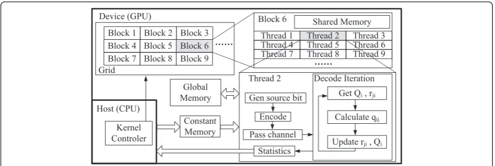
Figure 5 shows our GPU architecture. CPU is used as the controller, which puts the code into GPU constant memory, raises the GPU kernels and gets back the sta-tistics. While in GPU grid, we implement the whole coding system for each GPU block, including source generator, LDPC encoder, AWGN channel, LDPC deco-der and statistics. Our decoding algorithm is layered MMSA. In each GPU block, we assignzfthreads to cal-culate new LLRSUM and LLREX of thezf rows in each layer, wherezfis the expansion factor of QC LDPC. The zfthreads cooperate to complete the decoding job.
5.2. Algorithm and procedure
LMMSA for one row of this layer. The procedure ends up with the statistics ofP×QLDPC blocks.
5.3. Details and instructions
•Ensure“coalesced access”when reading or writing global memory, or the operation will be auto-serial-ized. In our algorithm, the adjacent threads should access adjacentL(Qi) andL(rji).
•Shared memory and registers are fast yet limited resources and their use should be carefully planned. In our algorithm, we storeL(Qi) in shared memory andL (rji) in registers due to the lack of resources.
•Make sure all theP×Qcores are running. This calls for careful assignment of limited resources (i.e., warps, shared memory, registers). In our case, we limit the registers per thread to 16 and threads per block to 128, or some of theQcores on each MP will“starve” and be disabled.
6. Hardware implementation schemes 6.1. Top-level hardware architecture
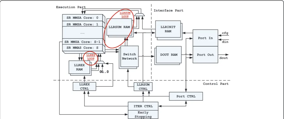
Our goal is to implement a multi-mode high-throughput QC-LDPC decoder, which can support multiple code rates and expansion factors on-the-fly. The proposed decoder consists of three main parts, namely, the interface part, the execution part and the control part. The top level architec-ture is shown in Figure 6.
The interface part buffers the input and output data as well as handling the configuration commands. In the execution part, the LLRSUM and LLREX are read out from the RAMs, updated in theΣparallel LMMSA cores, and written back to the RAMs, thus forming the LLRSUM loopand theLLREX loop, as marked red in Figure 6. The control part generates control signals, including port control, LLRSUM control, LLREX control and iteration control.
Note that thereconfigurable switch networkis designed in the LLRSUM loop to support multi-mode feature. As to achieve high-throughput, we propose thesplit-row MMSA core, the early-stopping scheme and the multi-block scheme. The split-row core has two data inputs and two data outputs, hence it also“splits”the LLRSUM RAM and LLREX RAM into two parts, meanwhile, two identical switch networks are needed to shuffle the data simulta-neously. We also propose theoffset-threshold decoding schemeto improve BER/BLER performance. The above five techniques are described in detail as follows.
6.2. The reconfigurable switch network
A switch network is anS-input,S-output hardware struc-ture that can put the input signals in the arbitrary order at the output. Formally, given input signalsx1,x2,...,xSwith data widthW, the output of switch network has the form
xa1,xa2, ...,xaS wherea1,a2,...,aSis any desired permutation of 1,2,...,S. For the design of reconfigurable LDPC deco-ders, two special kinds of output order are more impor-tant, described as follows.
•Full cyclic-shift:The output has the cyclic-shift form of the totalSinputs, i.e.,xc,xc+1,...xS, x1,x2...,xc −1, where 1≤c≤S.
•Partial cyclic-shift:The output has the cyclic-shift form of the firstpinputs, while other signal can be in arbitrary order, i.e., i.e.,xc,xc+1,...xp, x1,x2...,xc−1, x*,...x*, where 1 ≤ c<p<S, andx* can be any signal fromxp+1 toxS.
For the implementation of QC-LDPC decoder, the switch network is an essential module. Suppose
Hbj,i=Hbk,i≥0,j<k, and for any j<l<k, Hbl,i=−1, then the same data is involved in the processing of the above two “1"s, i.e., LLRSUM and LLREX of BNi × Zfto 'HYLFH *38
+RVW &38
.HUQHO &RQWUROHU
*OREDO 0HPRU\
%ORFN %ORFN %ORFN 7KUHDG 7KUHDG 7KUHDG
7KUHDG 7KUHDG 7KUHDG
7KUHDG 7KUHDG 7KUHDG
««
««
*HQ VRXUFH ELW
6KDUHG 0HPRU\
(QFRGH
3DVV FKDQQHO %ORFN
&RQVWDQW 0HPRU\
*HW 4L UML
&DOFXODWH TLM
8SGDWH UML 4L
'HFRGH ,WHUDWLRQ
6WDWLVWLFV 7KUHDG *ULG
%ORFN %ORFN %ORFN %ORFN %ORFN %ORFN
BN(i+1) × zf−1. However, after processing Hbj,i, the above data should be cyclic-shifted to ensure correct order for the processing Hb
j,k which corresponds tothe full cyclic-shiftcase with
S=zf, c= (Hvk,i−H b
j,i+S) mod S (9)
Further, in the case of multiple expansion factors, such as WiMAX [19] (zf = 24: 4: 96), thepartial cyclic-shiftis required with
S=zmaxf , p=zf, c= (Hkb,i−Hbj,i+p) modp (10)
The existing schemes to implement switch networks include the MS-CS network [20] and Benes network [13,21,22]. The former structure can handle the case when S is not a power of 2, while the latter is proved more efficient in area and gate count. In [13], the most efficient on-the-fly generation method of control signals is proposed. Therefore, we adopt the Benes network proposed in [13] for our decoder. The structure is shown in Figure 7 and the features is given in Table 1.
6.3. The offset-threshold decoding scheme
In this part, we propose the offset-threshold decoding method, which is adopted in our decoder architecture. Unlike existed modifications of MSA [5], the proposed scheme uses an offset-threshold correction to further improve the BER/BLER performance.
The traditional MSA is a simplified version of BP, by replacing the complicated Equation (2) with simple min operation, shown as follows.
sgn (L(rji)) =
⎛
⎝
i∈Rj\i
sgn (L(qij))
⎞
⎠ (11)
abs(L(rji)) = min
i∈Rj\i(L(qij)) (12) In [5], the normalized and offset MMSA schemes (13) (14) are proposed to compensate the loss of the above approximation, described as follows.
abs(L(rji)) =α·abs(L(rji)) (13)
abs(L(rji)) = max (abs(L(rji))−β, 0) (14)
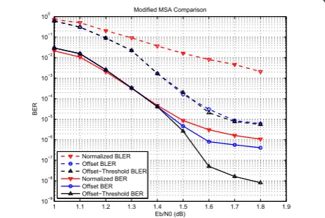
In our simulation, for BLER, the offset MMSA per-forms better than normalized one. However, as to BER, both schemes show error floor at 10−6, as shown in Figure 8. The problem here is that, for most cases, the offset MMSA works well, while in a few cases, the decoding fails with many bit errors in one block. The intuitive explanation of such phenomenon is existence of extremely large likelihoods (L(qij),L(rji)). In high SNR region, the L(qij) likelihoods converge fast to a large value, for both correct and wrong bits in some cases. The wrong bits not only remain wrong, but also propa-gate large L(rji) to other bits, resulting in more wrong bits and finally failure of decoding. For this reason, we need to set threshold upon offset MMSA to limit the likelihoods of becoming extremely large, which leads to the proposed offset-threshold scheme, done by the fol-lowing equation.
5$0B//5B (;
5$0B//5B68
0 5$0B//5B,1
,7
6KXIIOH QHW
//5(; &75/ ([HFXWLRQ3DUW
&RQWURO3DUW 3RUW,Q
3RUW&75/ ,QWHUIDFH3DUW
65006$&RUH
65006$&RUH
««
65006$&RUH6 6500$6&RUH6
FIJ
GLQ
GRXW
,7(5&75/ //5(;
5$0
6ZLWFK 1HWZRUN
//56805$0 //5,1,7
5$0
5$0B'287
//5680 &75/
'2875$0 3RUW2XW
(DUO\ 6WRSSLQJ
//5(; /223
//5680 /223
abs(L(rji)) = min (max(abs(L(rji))−β, 0),γ) (15)
The difference between traditional MSA, normalized MMSA, offset MMSA and offset-threshold MMSA is shown in Figure 9. Simulation result (Figure 8) shows that the proposed scheme has lowest error floor (10−8) among the above schemes, while achieving good BLER performance as offset MMSA.
6.4. The split-row MMSA core
This part presents the split-row MMSA core. In tradi-tional semi-parallel structure with layered MMSA core (see Figure 4), since the“1"s inj-th row will be processed one by one to find the minimum and sub-minimum of allL(qij), the decoding stagesKfor one iteration is pro-portional to the number of“1"s in each row of the base matrixHb. The idea is that, ifk“1"s can be processed at the same time, the decoding time of one iteration will be shortened by a factor ofk, and the throughput will have a gain ofk. This is done by split-row scheme, which verti-cally splitsHbinto multiple part. The“1"s in each part are processed simultaneously to find the local minimum, and the results are merged together. In this way, forHb with maximum row weightw, the minimum and sub-minimum can be obtained inw/kclocks. See Figure 2 as an example, we split the 4 × 6Hbinto two parts, each has one or two “1"s in every row. The corresponding
architecture with k = 2 is shown in Figure 10. The LLRSUM (L(Qi)), LLREX (L(rji)) and LLR (L(qij)) of the left part and right part are stored in two individual RAM/ FIFOs, respectively. Two minimum/sub-minimum fin-ders pass result to the merger for final comparison, thus approximately shorten the process pipeline by half. Note that the split position must exist for the codeHbsuch that each row in each part contains nearly the same num-ber of“1"s. Otherwise, we need RAMs with multiple read ports and write ports, which is not practical for FPGA implementation.
6.5. The early-stopping scheme
This part introduces the early-stoping scheme applied in our decoder. In practical scenario, the decoding process often gets to convergence much earlier than the preset maximum iterations is reached, especially under favor-able transmission conditions when SNR is large. Thus, if the decoder can terminate the decoding iterations as 6 ,QSXW
%HQHV 1HWZRUN
6 ,QSXW %HQHV 1HWZRUN
Ă
Ă
//5B
//5B
//5B6
//5B6 //5B
//5B
//5B6
//5B6
SF 6
&RQWURO 6LJQDO *HQHUDWLRQ 0RGXOH
Ă
Ă
Ă
Ă
//5BF
//5BF
//5B
//5B //5BF
//5BF
//5B
//5B
Figure 7The structure of Benes network.
Table 1 Features of reconfigurable Benes network Scale W= 9,S= 256, 15 stages, 128 × 15 MUX Support p= 64:8:256, 1≤c≤p
Resource 20866 LE, 388 memory bits
Clock 100 MHz for Cyclone II, 240 MHz for Stratix III Delay Two clocks for control signals, four clocks for output
1 1.1 1.2 1.3 1.4 1.5 1.6 1.7 1.8 1.9
10−9
10−8
10−7
10−6
10−5
10−4
10−3
10−2
10−1
100
Eb/N0 (dB)
BER
Modified MSA Comparison
Normalized BLER Offset BLER Offset−Threshold BLER Normalized BER Offset BER Offset−Threshold BER
soon as it detect the convergence, the power of the cir-cuit can be reduced as well as the decoding delay. Throughout is also increased if the system dynamically adjusts the transmission rate according to statistics of average iteration numbers under current channel state.
Traditional stopping criterions focus on whether the code can be decoded successfully or not, which either cost too much extra resource to store iteration parameters, such as HDA [23] and NSPC [24], or use floating-point calculation to evaluate the current iteration situation, such as VNR [25] and CMM [23]. All these methods are not suitable for the hardware implementation.
Here, we propose a simple and effective scheme to detect the convergence of the decoding. The“ conver-gence”means at some time, all of the hard decisions sgn (L(Qi)) satisfy the check equations, The detection of con-vergence usually demands parallel calculation of each equation, However, due to the layered structure (QC) and lack of the hardware resources, we can use a semi-parallel
algorithm to implement iteration-stopping module, which evaluates one layer (zfequations) simultaneously. If the number of the continuously successful-check layers reach a thresholdω, the module will trigger a signal meaning the decoding have got to convergence and the iteration can be stopped.
One important issue of Algorithm 5 is the estimation of thresholdω. The BER/BLER performances and average iteration times of differentω are shown in Figure 11, where the stopping criterion of ideal iteration isHcT= 0. We chooseω= 2.5 ×Mto achieve tradeoff between time and performance. In this case, if the average iteration times isIave(ideal iteration case), the decoding terminates at approximatelyIave+ 2 iterations.
6.6. The multi-block scheme
Suppose the LDPC code with code lengthNand expan-sion factorzf still has serious memory conflicts though being optimized by our SA and ACO algorithms, which is common for large zf and relatively small N. To address this problem, we propose a hardware method called“multi-block” to further avoid memory conflicts and increase pipeline efficiency. The “multi-block” scheme is explain as follows.
We construct a new matrix Hv by the parity-check matrixHwithMrows:
Hυ=
Here “virtual matrix” Hv is the combination of two codesHwithout“cross constraint” (edge between nodes from different codes in Tanner Graph) between each other. Suppose v1, v2 are any two legal encoded blocks satisfying that
Figure 9Comparison of the correction types of different MSA schemes.
Figure 10The architecture of split-row MMSA core.
1 1.2 1.4 1.6 1.8
BER in iteration termination
ω=2*M
Average iterations in termination
ω=2*M ω=2.5*M ω=3*M Ideal Iteration
v1.HT= 0 v2.HT= 0 (17)
The key observation is that there are no memory con-flicts between the two codesHdue to the diagonal form of Hv. This enables us to reorder and combine the decoding schedule of the two codes to reduce memory conflict of each code. We rewriteHandHvas follows:
H=
decoding schedule is given by above equation, i.e., H(1)i
comes first, followed by H(2)i , and then H(1)i+1, and so on so forth. The benefit of this“multi-block”scheme is that the insertion of H(2)i provides extra stages for the
con-flicts between H(1)i and H(1)i+1.
To sum up, the“multi-block”scheme changes any gap-lmemory conflict to gap-(2l−1), thus can improve the pipeline efficiency significantly. Meanwhile, it demands no extra logic resources (LE) for the design, but may double the memory bits for buffering two encoded blocks. Since the depth of memory is not fully used on our FPGA, the proposed method can make full use of it with no extra resource cost.
7. Numerical simulation
In this section, we show how our platform produces
“good”LDPC codes with outstanding decoding perfor-mance and hardware efficiency. For comparison, we tar-get on the WiMAX LDPC code (N= 2304, R= 0.5,zf= 96). We use the same parameters and degree distribu-tions as WiMAX for our SA-based constructor. We set
“cycle” as performance metric and memory conflict as efficiency metric. The performance of one of the candi-date codes and the WiMAX code are listed in Table 2. The candidate code has much less length-6/8 cycles and gap-1/2/3 memory conflict. Usually, the candidate codes can eliminate length-6 cycles and gap-1 conflicts, which ensures a larger-than-or-equal-to 8 girth and no conflict under short pipeline (whenK≤wm).
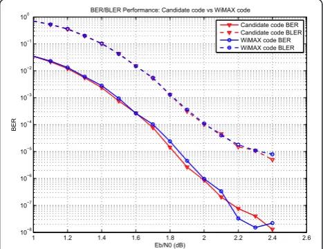
We simulate the candidate code and WiMAX code through the GPU platform. The BER/BLER performance is shown in Figure 12, while the platform parameters and throughput are listed in Table 3. The water-fall region and the error floor of our candidate code is almost the same as WiMAX code. For speed compari-son, we also include the fastest result that ever reported [12]. The “net throughput” is defined by the decoded
“message bits” per second, given by:
net throughput = P·Q·N·R
t (20)
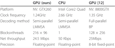
wheretis the consumed time for running through the GPU kernel (for us is Algorithm 4). As shown in Table 3, our GPU platform speeds up 490 times against CPU and achieves a net throughput 24.5 Mbps. Further, our throughput approaches the fastest one, while providing better precision (floating-point vs. 8 bit fixed-point) for the simulation.
Finally, we optimize the pipeline schedule by ACO-based scheduler, shown in Table 2. The“pipeline occu-pancy” is given by running/total clocks required for one iteration. For the candidate code, the number of idle clock insertions after ACO is 5, compared with 12 before ACO, achieving a 58.3% reduction. While for WiMAX code, 20 idle clock insertions remain required after layer-permutation-only (single-layer) scheme Table 2 Cycle and conflict performance of the two codes
Candidate code WiMAX code
Cycle:length 6/8 0/55 5/150
Conflict:gap 1/2/3 0/3/9 5/11/15 Pipeline occupancy Before ACO: 76/88 Only layer
After ACO: 76/81 permu.: 76/96
1 1.2 1.4 1.6 1.8 2 2.2 2.4 2.6
BER/BLER Performance: Candidate code vs WiMAX code
Candidate code BER Candidate code BLER WiMAX code BER WiMAX code BLER
proposed by [11]. In this case, the double-layered ACO achieves a 75% reduction against the single-layer scheme (5 vs. 20 idle clocks).
8. The multi-mode high-throughput decoder Based on the above techniques, namely,reconfigurable switch network,offset-threshold decoding,split-row MMSA core,early-stoping scheme andmulti-block scheme, we implement the multi-mode high-throughput LDPC deco-der on Altera Stratix III FPGA. The proposed decodeco-der supports 27 modes, including nine different code lengths and three different code rates, and maximum 31 iterations. The configurations for code length, code rate, and itera-tion number are completely on-the-fly. Further, it has a BER gap less than 0.2 dB against floating-point LMMSA, while achieving a stable net-throughput 721.58 Mbps under code rateR= 1/2 and 20 iterations (corresponding to a bit-throughput 1.44 Gbps). With early-stopping mod-ule working, the net-throughput can boost up to 1.2 Gbps (bit-throughput 2.4 Gbps), which is calculated under aver-age 12 iterations. The features are listed in Table 4.
One great advantage of the proposed multi-mode high-throughput LDPC decoder is that more modes can be supported with only more memory bits consumed and no architecture level change. Since thereconfigurable switch networksupports all expansion factorszf≤ 256, and the layered MMSA cores supports arbitrary
QC-LDPC codes, more code lengths and code rates are natu-rally supported, for example, the WiMAX codes (zf= 24: 4: 96,R= 1/2, 2/3, 3/4, 5/6, 114 modes in total). The only cost is that more memory bits are required to store the new base matricesHb.
9. Conclusion
In this article, a novel LDPC code construction, verifica-tion, and implementation methodology is proposed, which can produce LDPC codes with both good decoding perfor-mance and high hardware efficiency. Additionally, a GPU verification platform is built that can accelerate 490× speed against CPU and a multi-mode high-throughput decoder is implemented on FPGA, achieving a net-throughput 1.2 Gbps and performance loss within 0.2 dB.
Additional material
Additional file 1: Algorithm. This file contains Algorithm 1, Memory conflict minimization algorithm; Algorithm 2, ACO algorithm for TSP; Algorithm 3, The SA based LDPC construction framework; Algorithm 4, The GPU based LDPC simulation; and Algorithm 5, Semi-parallel early-stopping algorithm.
Acknowledgements
This paper is partially sponsored by the Shanghai Basic Research Key Project (No. 11DZ1500206) and the National Key Project of China (No. 2011ZX03001-002-01).
Competing interests
The authors declare that they have no competing interests.
Received: 15 May 2011 Accepted: 6 March 2012 Published: 6 March 2012
References
1. R Gallager, Low-density parity-check codes. IRE Trans. Inf. Theory.8(1), 21–28 (1962). doi:10.1109/TIT.1962.1057683
2. R Tanner, A recursive approach to low complexity codes. IEEE Trans. Inf. Theory.27(9), 533–547 (1981)
3. D MacKay, Good error-correcting codes based on very sparse matrices. IEEE Trans. Inf. Theory.45(3), 399–431 (1999)
4. T Richardson, M Shokrollahi, R Urbanke, Design of capacity approaching irregular low-density parity-check codes. IEEE Trans. Inf. Theory.47(2), 619–637 (2001). doi:10.1109/18.910578
5. J Chen, RM Tanner, C Jones, L Yan Li, Improved min-sum decoding algorithms for irregular LDPC codes, inProc. ISIT, (Adelaide, 2005), pp. 449–453 6. DE Hocevar, A reduced complexity decoder architecture via layered
decoding of LDPC codes, inIEEE workshop on SiPS, pp. 107–112 (2004) 7. Y Hu, E Eleftheriou, DM Arnold, Regular and irregular progressive edge
growth Tanner graphs. IEEE Trans. Inf. Theory.51(1), 386–398 (2005) 8. D Vukobratovic, V Senk, Generalized ACE constrained progressive
Eedge-growth LDPC code design. IEEE Comm. Lett.12(1), 32–34 (2008) 9. AJ Blanksby, CJ Howland, A 690-mW 1-Gb/s 1024-b, rate-1/2 low-density
parity-check code decoder. J. Solid State Circ.37(3), 404–412 (2002). doi:10.1109/4.987093
10. Z Cui, Z Wang, Y Liu, High-throughput layered LDPC decoding architecture. IEEE Trans. VLSI Syst.17(4), 582–587 (2009)
11. C Marchand, J Dore, L Canencia, E Boutillon, Conflict resolution for pipelined layered LDPC decoders, inIEEE workshop on SiPS, (Tampere, 2009), pp. 220–225
Table 3 Parameters and performance: GPU vs CPU (20 iterations)
GPU (ours) CPU GPU [12]
Platform NV. GTX260 Intel Core2 Quad NV. 8800GTX Clock frequency 1.24GHz 2.66 GHz 1.35 GHz Decoding method Semi-parallel Semi-parallel Full-parallel
LMMSA LMMSA BP
Blocks×threads 216 × 96 1 128 × 256 Net throughput 24.5 Mbps 50 Kbps 25Mbps Precision Floating-point Floating-point 8-bit fixed-point
Table 4 Features of the multi-mode high-throughput decoder
FPGA platform Altera Stratix III EP3SL340F1517C2 Decoding scheme Layered offset-threshold MSA Modes supported 9 × 3 = 27 modes
Code length N= 1536:768:6144 (zf= 64:32:256) Code rate R= 1/2,2/3,3/4 (Hb:12 × 24, 8 × 24, 6 × 24) Iteration number iter = 1−31, 20 recommended
Resources usage 149, 976 LE, 3, 157, 136 bits memory BER performance gap≤0.2 dB vs. 20 iteration float LMMSA Clock setup 225.58MHz
12. G Falcao, V Silva, L Sousa, How GPUs can outperform ASICs for fast LDPC decoding, inProc. international conf on Supercomputing, (New York, 2009), pp. 390–399
13. J Lin, Z Wang, Effcient shuffle network architecture and application for WiMAX LDPC decoders, inIEEE Trans. on Circuits and Systems.56(3), 215–219 (2009)
14. KK Gunnam, GS Choi, MB Yeary, M Atiquzzaman, VLSI architectures for layered decoding for irregular LDPC codes of WiMax, inIEEE International Conference on Communications, (Glasgow, 2007), pp. 4542–4547 15. T Brack, M Alles, F Kienle, N Wehn, A synthesizable IP core for WIMAX
802.16E LDPC code decodings, inIEEE Inter. Symp. on Personal, Indoor and Mobile Radio Comm, (Helsinki, 2006), pp. 1–5
16. K Tzu-Chieh, AN Willson, A flexible decoder IC for WiMAX QC-LDPC codes, inCustom Integrated Circuits Conference, (San Jose, 2008), pp. 527–530 17. M Dorigo, LM Gambardella, Ant colonies for the travelling salesman
problem. Biosystems.43(2), 73–81 (1997). doi:10.1016/S0303-2647(97)01708-5
18. S Kirkpatrick, CD Gelatt, MP Vecchi, Optimization by simulated annealing. Science, New Series.220(4598), 671–680 (1983)
19. IEEE Standard for Local and Metropolitan Area Networks Part 16. IEEE Standard 802.16e (2008)
20. M Rovini, G Gentile, F Rossi, Multi-size circular shifting networking for decoders of structured LDPC codes. Electron Lett.43(17), 938–940 (2007). doi:10.1049/el:20071157
21. J Tang, T Bhatt, V Sundaramurthy, Reconfigurable shuffle network design in LDPC decoders,IEEE Intern Conf ASAP, (Steamboat Springs, CO, 2006), pp. 81–86 22. D Oh, K Parhi, Area efficient controller design of barrel shifters for
reconfigurable LDPC decoders, inIEEE Intern Symp on Circuits and Systems, (Seattle, 2008), pp. 240–243
23. L Jin, Y Xiao-hu, L Jing, Early stopping for LDPC decoding: convergence of mean magnitude (CMM). IEEE Commun Lett.10(9), 667–669 (2006). doi:10.1109/LCOMM.2006.1714539
24. S Donghyuk, H Kyoungwoo, O Sangbong, A Jeongseok Ha, A stopping criterion for low-density parity-check codes, inVehicular Technology Conference, (Dublin, 2007), pp. 1529–1533
25. F Kienle, N Wehn, Low complexity stopping criterion for LDPC code decoders, inVehicular Technology Conference.1, 606–609 (2005)
doi:10.1186/1687-1499-2012-84
Cite this article as:Yuet al.:Systematic construction, verification and implementation methodology for LDPC codes.EURASIP Journal on Wireless Communications and Networking20122012:84.
Submit your manuscript to a
journal and benefi t from:
7Convenient online submission 7Rigorous peer review
7Immediate publication on acceptance 7Open access: articles freely available online 7High visibility within the fi eld
7Retaining the copyright to your article