A complex path around the sign problem

A complex path around the sign problem

Paulo F. Bedaque1,

1_{University of Maryland, College Park 20742 MD USA}

Abstract.We review recent attempts at dealing with the sign problem in Monte Carlo calculations by deforming the region of integration in the path integral from real to com-plex fields. We discuss the theoretical foundations, the algorithmic issues and present some results for low dimensional field theories in both imaginary and real time.

1 Introduction

The Monte Carlo approach to field theories is based on the path integral representation of the expec-tation of operators given by the path integral:

O=

DφeiS_O(φ)

DφeiS , (1)

whereφstands for the fields in the theory andS is the action of the theory. After discretization the integral in eq.(1) becomes a finite dimensional integral. The numerical computation of an integral of this type is nearly impossible due to the highly oscillatory integrand. The standard procedure to deal with this problem is to use a Wick rotation of the time coordinatet→itwhich transforms the integral into

O= Dφe −S_O(φ)

Dφe−S , (2)

where nowS stands for the euclidean action. In many cases of interest, the euclidean actionS is a real quantity. In this case the integral in eq.(2) has the form of a classical thermodynamic average and it can be evaluated by Monte Carlo methods usingimportance sampling.Ois estimated as

O ≈ 1 N

N

a=1

O(φ()), (3)

whereφ(a), a = 1,· · · ,N are a set of field configurations distributes according to the probability distributionP[φ] ∼ eS[φ]_{. However, there are many other cases of physical interest in which the} euclidean action is not real. In that case, the Monte Carlo method can still be used if one separates the

real and imaginary parts of the action asS =SR+iSI and considering the phasee−iSI as part of the

observable with the help of the equation:

O=

Dφe−S_O

Dφe−S =

Dφe−SR_Oe−iSI

Dφe−SR

Dφe−SR

Dφe−SRe−iSI =

Oe−iSI_SR

e−iSI_S R

. (4)

This method (“reweigthing") works to the extend that the average phasee−iSI_SRis not small and the

expectation value does not result from a ratio of very small numbers. In the thermodynamic limit (and at low temperature), where the spacetime volumeβVdiverges, the fluctuations ofSIalso diverges and

the average sign decreases exponentially asβVgrows. This is the sign problem.

Physical systems with sign problems include some of the most interesting physics problems. Sys-tems at finite density typically suffer from the sign problem. That includes the study of cold, dense hadronic/quark matter, a central problem in nuclear physics and astrophysics. Many models used in condensed matter models, like the Hubbard model away from half-filling, also have a sign problem. In addition, the direct evaluation of time-dependent quantities, even in thermal equilibrium, based on real time integrals like in eq.(1), lead to integrals like the one in eq.(1) and have a particularly nasty sign problem1_{. Given the importance of all these physical systems it is no surprise that many} ideas have been put forward to solve or ameliorate the sign problem, too many to even mention (some reviews can be found in [1–4]). There is even an argument showing that the sign problem is a NP-complete problem in at least one specific model, implying that a general solution to the sign problem is extremely unlikely to be found [5].

For one-dimensional integrals, there is a well know way of dealing with the oscillatory integrals leading to the sign problem: the stationary phase of steepest descent method. In the stationary phase method one changes the contour of integration in the integral dz e−S _{from the real axis to a}

con-tour on the real plane going through one (or perhaps more) critical points (defined by the condition S_{(z)=0) such that the phase of the integrand is constant. Since the change of contour, under some} circumstances, does not alter the value of the integral, this change of contour provides a way of computing the original integral without having to deal with oscillatory phases. The stationary phase contour has one extra feature: it goes along the direction where the absolute value of the integrand decreases the fastest, hence the alternative name “steepest descent" for this contour. This makes the stationary phase/steepest descent contour also ideal for semi-classsical evaluations of the integral and it is in this context that it is better known among physicists. For the resolution of the sign problem however, it is the constant phase of the integrand on this contour that is relevant.

In this proceeding we will discuss a recent approach to the solution to the sign problem that can be viewed as an extension of the stationary phase/steepest descent contour method, but the method does not involve any semi-classical expansion. It is based on deforming the manifold of integration from real variablesRNto another N-dimensional manifold embedded on the complexified field space CN. There are at this point in time a variety of choices for the precise deformation of the manifold of integration to be used. Even larger is the choice of algorithmic ideas suggest to accomplish the task in practice. We will discuss some mathematical generalities related to the change of manifolds of integration in section2, one algorithm (and its variations) to compute the path integral in practice in section3and present two examples of the method in action in section4. In the final section we briefly comment on newer ideas and future prospects.

1_{In thermal equilibrium, real time correlators can be obtained form an analytic continuation of imaginary time correlators}

real and imaginary parts of the action asS =SR+iSIand considering the phasee−iSI as part of the

observable with the help of the equation:

O=

Dφe−S_O

Dφe−S =

Dφe−SR_Oe−iSI

Dφe−SR

Dφe−SR

Dφe−SRe−iSI =

Oe−iSI_S R

e−iSI_S R

. (4)

This method (“reweigthing") works to the extend that the average phasee−iSI_SRis not small and the

expectation value does not result from a ratio of very small numbers. In the thermodynamic limit (and at low temperature), where the spacetime volumeβVdiverges, the fluctuations ofSIalso diverges and

the average sign decreases exponentially asβVgrows. This is the sign problem.

Physical systems with sign problems include some of the most interesting physics problems. Sys-tems at finite density typically suffer from the sign problem. That includes the study of cold, dense hadronic/quark matter, a central problem in nuclear physics and astrophysics. Many models used in condensed matter models, like the Hubbard model away from half-filling, also have a sign problem. In addition, the direct evaluation of time-dependent quantities, even in thermal equilibrium, based on real time integrals like in eq.(1), lead to integrals like the one in eq.(1) and have a particularly nasty sign problem1_{. Given the importance of all these physical systems it is no surprise that many} ideas have been put forward to solve or ameliorate the sign problem, too many to even mention (some reviews can be found in [1–4]). There is even an argument showing that the sign problem is a NP-complete problem in at least one specific model, implying that a general solution to the sign problem is extremely unlikely to be found [5].

For one-dimensional integrals, there is a well know way of dealing with the oscillatory integrals leading to the sign problem: the stationary phase of steepest descent method. In the stationary phase method one changes the contour of integration in the integral dz e−S _{from the real axis to a}

con-tour on the real plane going through one (or perhaps more) critical points (defined by the condition S_{(z)=0) such that the phase of the integrand is constant. Since the change of contour, under some} circumstances, does not alter the value of the integral, this change of contour provides a way of computing the original integral without having to deal with oscillatory phases. The stationary phase contour has one extra feature: it goes along the direction where the absolute value of the integrand decreases the fastest, hence the alternative name “steepest descent" for this contour. This makes the stationary phase/steepest descent contour also ideal for semi-classsical evaluations of the integral and it is in this context that it is better known among physicists. For the resolution of the sign problem however, it is the constant phase of the integrand on this contour that is relevant.

In this proceeding we will discuss a recent approach to the solution to the sign problem that can be viewed as an extension of the stationary phase/steepest descent contour method, but the method does not involve any semi-classical expansion. It is based on deforming the manifold of integration from real variablesRNto another N-dimensional manifold embedded on the complexified field space CN. There are at this point in time a variety of choices for the precise deformation of the manifold of integration to be used. Even larger is the choice of algorithmic ideas suggest to accomplish the task in practice. We will discuss some mathematical generalities related to the change of manifolds of integration in section2, one algorithm (and its variations) to compute the path integral in practice in section3and present two examples of the method in action in section4. In the final section we briefly comment on newer ideas and future prospects.

1_{In thermal equilibrium, real time correlators can be obtained form an analytic continuation of imaginary time correlators}

obtained form integrals like eq.(2). The analytic continuation of noise numerical data is, however, exponentially hard due to numerical instabilities.

2 Complexified fields, thimbles, anti-holomorphic flow

O=

dφie−S[φ]O[φ]

dφie−S[φ]

. (5)

By a generalization of the Cauchy theorem familiar from complex analysis, the same integrals can be obtained by integrating over an N-dimensional submanifoldMofCN parametrized byφi =φi(ζj), i,j=1,· · ·N:

Z=

RNdφie

−S[φ]_O[φ]= Mdφie

−S[φ]_{O[φ]= dζ}

idet

∂φi

∂ζj

e−S[φ(ζ)]_{, (6)}

whereφiis now a complex variable,ζjare the real variables parametrizing the manifoldM,S[φ(ζ)]

is the analytic continuation of the action and detJ =det

∂φi ∂ζj

is the jacobian related to the change of variables fromφitoζj. Notice thatφiare complex and so is the jacobianJ.

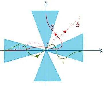
The change of domain of integration fromRN toMdoes not necessarily lead to the same value of the integrals and care must be taken when performing this step. In the theory of complex functions of one variable the rule determining which deformations do not change the value of the integral are well known: the deformations allowed are the ones that can be made continuously from the initial to the final contour without crossing any singularity (pole, branch cut) of the integrand including “poles at infinity". When poles are crossed during the deformation the value of the integrand jumps discontinuously. For contours extending towards the infinity the integral is not even necessarily well defined. In fact, the integral exists only for contours that approach the point at infinity along certain directions. For the other directions, the integrand does not decay to zero fast enough and the integral diverges. This can be exemplified with the help of the integral_−∞∞ dz e−z4

. This integral only exists for contours beginning and ending along the shaded regions on fig.2. Since the integrand has no singularity at finite values ofzwe are free to move the contour around as long as the its beginning and end of the contour do not jump from one of the shaded regions to another. Doing that amounts to crossing the singularity atz = ∞. Thus, the real line is equivalent to the contour labelled 1 but differs from the one labelled 2. The integral is not even defined on the contour 3. Notice that in order to deform contour 1 into contour 2, the end of the contour has to necessarily pass through a region where the integrral diverges. Two contour are said to be equivalent if they lead to the same value of the integral. The set of all contours (in which the integral is well defined) can thus be divided up in equivalent classes (homology classes) dependent only on which of the shaded regions the initial and final points of the contour lie.

The integrands encountered in lattice field theory do not typically have any singularities. For the most part they are exponential of polynomials (the Boltzmann factore−S _{), perhaps multiplied by}

another polynomial (observables and/or fermion determinants)2. In theories where the field vari-ables are compact (before complexification), the absence of singularities on the integrand is enough to guarantee that any continuous deformation of the domain of integration does not alter the value of the integral. In theories where the fields take values on a non-compact region, likeRNthere may be singularities at asymptotically large values of the fields. Just like one-dimensional integrals, the integrand is well defined only if the asymptotic values are approached from certain “good" directions. 2_{The formal integration over fermion fields lead to the appearance of propagators computed on the background of bosonic}

Figure 1.The integral dz e−z4

is only well defined for contours approaching the infinity along the shaded (blue) areas. The integral over contour 1 is equivalent to the integral overR. Contour 2 leads to a different result while the integral over contour 3 is divergent and not well defined. A continuous deformation of contours fromRto contour 2 necessarily passes through contours where the integral diverges. This general pattern remains true in higher dimensions.

And like one dimensinonal integrals, the set of “good" directions are grouped in discrete sets (homol-ogy classes) and the integral takes on a different value in each of these groups [6–10]. As the domain of integration is changed in such a way to make the asymptotic regions go from one “good direction" to another, the value of the integral jumps discontinuously (a “pole at the infinity" was crossed). In between two “good regions" the integral diverges. Thus, a sufficient condition for a deformation not to change the value of the integral is that it can be continuously connected with the initial domain of integration and that, at all intermediate steps of the deformation, the integral is well defined. This conditions guarantee that the domains lie in the same homology class and can be used as a integration domain instead of the originalRN.

Now that we know that the domain of integration can be moved to a different one in complex

space the question is whether this is advantageous. For instance, we may look for aN−dimensional

manifoldM embedded in CN on which the phase e−iSI is constant. In fact, the condition S_{I =}

constant is one single condition on a function of 2Nreal variables, defining a 2N−1 submanifold of

CN =R2N; there are certainly manyN dimensional manifolds in that 2n−1 dimensional subspace.

But not all manifoldsMwheree−iSI is constant is suitable. For instance, if the Boltzmann factore−SR

defines a complicated multimodal landscape onMsuch a manifold will be unsuitable for Monte Carlo

Figure 1.The integral dz e−z4

is only well defined for contours approaching the infinity along the shaded (blue) areas. The integral over contour 1 is equivalent to the integral overR. Contour 2 leads to a different result while the integral over contour 3 is divergent and not well defined. A continuous deformation of contours fromRto contour 2 necessarily passes through contours where the integral diverges. This general pattern remains true in higher dimensions.

And like one dimensinonal integrals, the set of “good" directions are grouped in discrete sets (homol-ogy classes) and the integral takes on a different value in each of these groups [6–10]. As the domain of integration is changed in such a way to make the asymptotic regions go from one “good direction" to another, the value of the integral jumps discontinuously (a “pole at the infinity" was crossed). In between two “good regions" the integral diverges. Thus, a sufficient condition for a deformation not to change the value of the integral is that it can be continuously connected with the initial domain of integration and that, at all intermediate steps of the deformation, the integral is well defined. This conditions guarantee that the domains lie in the same homology class and can be used as a integration domain instead of the originalRN.

Now that we know that the domain of integration can be moved to a different one in complex

space the question is whether this is advantageous. For instance, we may look for aN−dimensional

manifold M embedded in CN on which the phase e−iSI is constant. In fact, the condition S_{I =}

constant is one single condition on a function of 2Nreal variables, defining a 2N−1 submanifold of

CN =R2N; there are certainly manyNdimensional manifolds in that 2n−1 dimensional subspace.

But not all manifoldsMwheree−iSI is constant is suitable. For instance, if the Boltzmann factore−SR

defines a complicated multimodal landscape onMsuch a manifold will be unsuitable for Monte Carlo

calculations despite the absence of a sign problem. We will first show, as a proof of principle, that manifolds with constant phase and well behaved probability landscapes exist. This construction can be thought out as a multidimensional generalization of the steepest descent/stationary phase contour of one-dimensional integrals.

2.1 Anti-holomorphic flow and thimbles

Consider theanti-holomorphicflow defined by the equations3

dφi dt =

∂S

∂φi, (7)

where the bar denotes complex conjugation. The important property of the flow is that it increases the real part of the action while keeping the imaginary part constant. In fact,

dS dt =

∂S ∂φi

dφi dt =

∂S ∂φi

∂S ∂φi =

_∂φ∂S_i

2

≥0. (8)

This property can also be seen by splitting the flow in its real and imaginary part we can see that it is the gradient flow for the real part of the actionSRand the hamiltonian flow for the “hamiltonian"SI.

The flow has some critical (fixed) pointsφ0where∂S/∂φi=0, which we will assume to be isolated.

We can understand the behavior of the flow around a critical point by looking at its linearized form:

d∆φi

dt =Hi j∆φj, (9)

where∆φ=φ₋φ0is the displacement from the critical point andHi j= _∂φ∂2_i∂φS_j|φ=φ0is the hessian. The

linearized equations have the solutions

φi(t)=φ0i +

2N

a=1

eλat_ea

i, (10)

where the vectorsea_{and its “eigenvalues" satisfy:}

Hi jeaj=λaeai, (11)

with realλa(other solution exist with complexλa). It can be shown that

• λa,eacome in pairs: (λa,ea) and (−λa,iea) . We will assume that critical point are non-degenerate, that is, all eigenvalues ofHare non zero.

• ea_{form an orthogonal set:} 1

2(eaiebi +eaiebi)=δab.

• any complex vector inCNcan be written as a real linear combination of theea_asv=2N

a=1Aaeaor

as a complex linear combination of theea_{with positive eigenvalues asv=}N

a=1(Aa+iBa)ea.

From eq.(10) we see that the flow around a critical point is repulsive along N of the 2N (real) directions, the ones given by the eigenvectorsea_{with positiveλ}a_{. The flow is attractive along the other}

Ndirections. The points reached by the flow along the repulsive directions form the thimbleof the

critical point. It follows from the properties of the flow that the imaginary part of the action is constant on the thimble and that the real part of the action grows monotonically as the flow moves away from the critical point. As such, thimbles are the proper generalization of the steepest descent/stationary phase contour to the many dimensional case.

In general, there are many critical points and corresponding thimbles and the original integral over real fields equals to the integral over a certain combination of thimbles. There is a recipe to determine whether a particular thimble is part of this combination: a particular thimble is part of the

combination of thimbles equivalent toRNis, by evolution of that thimble by thereverseflow intersects the original integration domain (RN_{). An intuitive argument for this statement will be presented on}

the next subsection.

The idea of using thimbles as the integration region in order to solve the sign problem in path integrals was put forward in [11]. There are two main problems in transforming this idea into a practical method:

1. There is no local characterization of the points belonging to a thimble so there is no obvious, computationally cheap way of making Monte Carlo proposals that lie on the thimble.

2. Except for the simplest toy models it is impossible to find all critical points, their thimbles and to determine which thimbles contribute to the original integral.

Problem number 1 has been addressed with several algorithmic ideas. One is the solution of the Langevin equation on the curved thimble, with an appropriate way of projecting the noise term on the tangent plane to the thimble [12]. The projection is the computationally most expensive part of the algorithm. A second method is an adaptation of the hybrid Monte Carlo algorithm to sampling on a thimble [13]. Here again the difficult and expensive part is the projection that guarantees the Monte Carlo chain stays on the thimble. The third method, which we will describe in more detail on the next section, uses a map of the thimble (in fact, all the relevant thimbles) by points onRN. An effective action on the space of real fields is then used with some standard method, like the Metropolis-Hastings algorithm. This last approach has the advantage of being able, in principle, of computing the integral over all the relevant thimbles at once, even if the existence and location of these thimbles is not known a priori.

Regarding the problem 2 above, it has been argued [11] using universality arguments that the integral over a single thimble is likely to agree with the full result in the continuum limit. Also, the contribution of every thimble is suppressed by a Boltzmann factore−S0

R, whereS0 is the the action

at the critical point, and one can imagine that at weak coupling or for large spacetime volumes the integral will be dominated by a single thimble. It is, however, very hard to put any of these arguments on a firm footing. The contribution of a thimble depends not only one−SRbut also on its “entropy". As

the spacetime volume increases or the lattice spacing decreases the position and number of thimbles changes. Finally, there is a phasee−iS0

I multiplying the contribution of each thimble; the contribution

of several thimbles may cancel or, if many thimbles contribute significantly, a sign problem might reappear when combining their contributions. The plausibility of the one thimble dominance can also be gauged against some of its consequences. In QCD, for instance, an instanton configuration is a solution of the classical equations of motion and so there is a thimble associated with it. If the thimble associated with the trivial configuration dominates the partition function, the instanton contributions and its physical consequences have to disappear in the infinite volume/continuum limits. Fortunately, there are ways to proceed without making any assumptions about the dominance of one or more thimbles and, in fact, those arguments can be tested with numerical calculations. The few examples where the thimble structure was fully understood do not have a continuum or thermodynamics limit where these questions ca be addressed [14–18].

2.2 Flowing towards the right thimbles

Consider taking every pointζofRNand evolving them by the flow in eq.(7) by a fixed timeT. The end pointsφT(ζ) of the trajectories form aN−dimensional manifold we callMT. Assuming the integrand

combination of thimbles equivalent toRNis, by evolution of that thimble by thereverseflow intersects the original integration domain (RN_{). An intuitive argument for this statement will be presented on}

the next subsection.

The idea of using thimbles as the integration region in order to solve the sign problem in path integrals was put forward in [11]. There are two main problems in transforming this idea into a practical method:

1. There is no local characterization of the points belonging to a thimble so there is no obvious, computationally cheap way of making Monte Carlo proposals that lie on the thimble.

2. Except for the simplest toy models it is impossible to find all critical points, their thimbles and to determine which thimbles contribute to the original integral.

Problem number 1 has been addressed with several algorithmic ideas. One is the solution of the Langevin equation on the curved thimble, with an appropriate way of projecting the noise term on the tangent plane to the thimble [12]. The projection is the computationally most expensive part of the algorithm. A second method is an adaptation of the hybrid Monte Carlo algorithm to sampling on a thimble [13]. Here again the difficult and expensive part is the projection that guarantees the Monte Carlo chain stays on the thimble. The third method, which we will describe in more detail on the next section, uses a map of the thimble (in fact, all the relevant thimbles) by points onRN. An effective action on the space of real fields is then used with some standard method, like the Metropolis-Hastings algorithm. This last approach has the advantage of being able, in principle, of computing the integral over all the relevant thimbles at once, even if the existence and location of these thimbles is not known a priori.

Regarding the problem 2 above, it has been argued [11] using universality arguments that the integral over a single thimble is likely to agree with the full result in the continuum limit. Also, the contribution of every thimble is suppressed by a Boltzmann factore−S0

R, whereS0 is the the action

at the critical point, and one can imagine that at weak coupling or for large spacetime volumes the integral will be dominated by a single thimble. It is, however, very hard to put any of these arguments on a firm footing. The contribution of a thimble depends not only one−SR_{but also on its “entropy". As}

the spacetime volume increases or the lattice spacing decreases the position and number of thimbles changes. Finally, there is a phasee−iS0

I multiplying the contribution of each thimble; the contribution

of several thimbles may cancel or, if many thimbles contribute significantly, a sign problem might reappear when combining their contributions. The plausibility of the one thimble dominance can also be gauged against some of its consequences. In QCD, for instance, an instanton configuration is a solution of the classical equations of motion and so there is a thimble associated with it. If the thimble associated with the trivial configuration dominates the partition function, the instanton contributions and its physical consequences have to disappear in the infinite volume/continuum limits. Fortunately, there are ways to proceed without making any assumptions about the dominance of one or more thimbles and, in fact, those arguments can be tested with numerical calculations. The few examples where the thimble structure was fully understood do not have a continuum or thermodynamics limit where these questions ca be addressed [14–18].

2.2 Flowing towards the right thimbles

Consider taking every pointζofRNand evolving them by the flow in eq.(7) by a fixed timeT. The end pointsφT(ζ) of the trajectories form aN−dimensional manifold we callMT. Assuming the integrand

has no singularities and the flow by timeT is well defined for all initial conditions with finite values of the fields, the multidimensional Cauchy theorem applies and the equality of the integrals hinges on

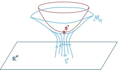
Figure 2. The flow takes point inRN _{to points inMT. The integral overMT equals the one overR}N _{at all} values ofT. AsT increases,MT approaches the combination of thimbles equivalent to the original domain of integration.

the singularities “at the infinity", that is, whether the two manifolds are in the same homology class. In many field theories of physical interest, like gauge theories andσ−models, the field variables are compact, the original domain of integration is notRN but some otherN−dimensional compact manifoldM0and there are not asymptotic directions where the integral might diverge. The integral overMT thus equals the one overM0. In the case of non-compact field variables we note that the

flow monotonically increases the real part of the action and, consequently, decreases the weighte−SR.

Since the integral was well defined overRN and the integrand only decreases asT increases, it is reasonable to assume that the integral remains finite and well defined for all intermediate values ofT. Since the value of the integral can only change, as the manifold on integration changes, after going through a region where the integral diverges (at large values of the field), we conclude that the integral will not change in the non-compact case either.

We can now find out what happens to the manifold MT as T is increased. One pointζ0 will

approach the critical pointφ0 asymptotically (if there isn’t such aζ0 that particular thimble is not

part of the set contributing to the original integral). The surrounding points will flow towards points with larger and larger values ofSR. However, no point can cross a thimble since the flow is tangent

to them. They can only asymptotically approach the thimbles. As a result, the flow “automatically" maps the real fields into a manifold that is close to the right combination of thimbles equivalent to the integration overRN. AsTis increased,MTbecomes closer to the thimbles. This situation is pictured

in fig.2.

There is a jacobian involved in the parametrization ofMT in terms of the real fields (the initial

conditions of the flow). If the result of flowing the pointζiby a timeT is the (complex) pointφi(ζ),

the jacobianJ=det(∂φi(ζ)/∂ζj) can be computed by taking a basis (v(a)) ofRNand evolving each of

its vectors by the flow

dv(_ia)

dt =

∂2_S

∂zi∂zkv

(a)

The computation of the jacobian is extremely expensive. Not onlyNsets ofNcomputed differential equations need to be solved but the determinant of aN×Ndense complex matrix need to be computed, leading to a computational cost of orderN34_{. Also, the jacobian is, in general, a complex number:} J = |J|eiα. A Monte Carlo evaluation of an integral overMT requires then the reweighting of the

“residual phase"αas well ase−iSI:

O=

MT Dφe

−S_O

MTDφe

−S =

Dφe−SR+log|J|_Oe−iSI+iα

Dφe−SR+log|J|

Dφe−SR+log|J|

Dφe−SR+log|J|e−iSI+iα =

Oe−iSI+iα SR

e−iSI+iα SR

. (13)

At large values ofT, the manifold MT is close to the (correct set of) thimbles and, sinceSI is a

constant over each thimble we don’t expectSIto fluctuate much unless many thimbles with different

phases contribute almost equally to the integral. Experience shows also that for the variety of models and parameter space studied up to now the residual phase also fluctuates little and there is no practical problem in reweighting it.

For weakly coupled theories (not necessarily perturbative) this is expected. In fact, free theories, which have a quadratic action, have flat thimbles with constantα. The experience accumulated

inves-tigating several models over a large swatch of parameters space suggests that the fluctuation ofαand,

for large enough flow timeT, the fluctuations ofSIalso, are small and easily reweigthed. Of course,

this always has to be verified in a particular calculation. An important theoretical question is whether this experience will extend to the continuum and infinite volume limits in 4 dimensional theories.

3 The generalized thimble method

3.1 Basic algorithm

The observations made in the previous sections suggest a way of computing the integral over a mani-foldMTin the same homology class asRN. This set of manifolds includes, if one takes a large enough

flowing timeT, the correct combination of thimbles equivalent to the real field space. The idea is to parametrize each pointφinMT by the pointζinRNthat flows to it: φ=φT(ζ), whereφT(ζ) is the

map given by flowingζ by a timeT. This way the action onMT can be thought of as a function of

the real fieldζ,S =S[φT(ζ)]. The jacobian can also be written in terms of the real variablesζ and

the simulation overMT is equivalent to a simulation over real fieldsζwith an effective action equal

toSe f f =S[z(ζ)]−log detJ(ζ). SinceSe f f is complex, its imaginary part needs to be reweighted, as

shown in eq.(13). The sampling of configurationsζi with distributionP[ζ]∼ e−Re(Se f f) can be done

with any of a number of methods like, for instance, the Metropolis algorithm. To summarize, the algorithm we propose is [20,21]:

1. Start from a initial pointζinRNand the corresponding effective actionS[φT(ζ)]−log detJ(ζ)

whereφT(ζ) is obtained by integrating the flow equations eq.(7) withζas the initial conditions

and solving eq.(9).

2. Make a random proposalζ =ζ+ ∆ζinRN and compute the corresponding pointφ=φT(ζ)

and compute the actionS[φ], the jacobianJ(ζ) and the effective actionS[φ]−log detJ(ζ).

3. Accept or reject the new configurationζbased on the real part of difference of effective actions between pointsζandζwith the usual Metropolis probabilities.

The computation of the jacobian is extremely expensive. Not onlyNsets ofNcomputed differential equations need to be solved but the determinant of aN×Ndense complex matrix need to be computed, leading to a computational cost of orderN34_{. Also, the jacobian is, in general, a complex number:} J = |J|eiα. A Monte Carlo evaluation of an integral overMT requires then the reweighting of the

“residual phase"αas well ase−iSI:

O=

MTDφe

−S_O

MTDφe

−S =

Dφe−SR+log|J|_Oe−iSI+iα

Dφe−SR+log|J|

Dφe−SR+log|J|

Dφe−SR+log|J|e−iSI+iα =

Oe−iSI+iα SR

e−iSI+iα SR

. (13)

At large values ofT, the manifold MT is close to the (correct set of) thimbles and, sinceSI is a

constant over each thimble we don’t expectSI to fluctuate much unless many thimbles with different

phases contribute almost equally to the integral. Experience shows also that for the variety of models and parameter space studied up to now the residual phase also fluctuates little and there is no practical problem in reweighting it.

For weakly coupled theories (not necessarily perturbative) this is expected. In fact, free theories, which have a quadratic action, have flat thimbles with constantα. The experience accumulated

inves-tigating several models over a large swatch of parameters space suggests that the fluctuation ofαand,

for large enough flow timeT, the fluctuations ofSI also, are small and easily reweigthed. Of course,

this always has to be verified in a particular calculation. An important theoretical question is whether this experience will extend to the continuum and infinite volume limits in 4 dimensional theories.

3 The generalized thimble method

3.1 Basic algorithm

The observations made in the previous sections suggest a way of computing the integral over a mani-foldMTin the same homology class asRN. This set of manifolds includes, if one takes a large enough

flowing timeT, the correct combination of thimbles equivalent to the real field space. The idea is to parametrize each pointφinMT by the pointζ inRN that flows to it:φ=φT(ζ), whereφT(ζ) is the

map given by flowingζ by a timeT. This way the action onMT can be thought of as a function of

the real fieldζ,S =S[φT(ζ)]. The jacobian can also be written in terms of the real variablesζ and

the simulation overMT is equivalent to a simulation over real fieldsζwith an effective action equal

toSe f f =S[z(ζ)]−log detJ(ζ). SinceSe f f is complex, its imaginary part needs to be reweighted, as

shown in eq.(13). The sampling of configurationsζi with distributionP[ζ] ∼e−Re(Se f f)can be done

with any of a number of methods like, for instance, the Metropolis algorithm. To summarize, the algorithm we propose is [20,21]:

1. Start from a initial pointζinRNand the corresponding effective actionS[φT(ζ)]−log detJ(ζ)

whereφT(ζ) is obtained by integrating the flow equations eq.(7) withζas the initial conditions

and solving eq.(9).

2. Make a random proposalζ=ζ+ ∆ζinRN and compute the corresponding pointφ=φT(ζ)

and compute the actionS[φ], the jacobianJ(ζ) and the effective actionS[φ]−log detJ(ζ).

3. Accept or reject the new configurationζbased on the real part of difference of effective actions between pointsζandζwith the usual Metropolis probabilities.

4_{A method for the computation of the residual phase is discussed in [19]}

4. Return to 2 until a suitably large number of (statistically independent) configurations is col-lected.

5. Compute the average of the phasee−iSI+iα _{and the observableOe}−iSI+α_{over the collected}

con-figurations using the imaginary parts of the action (ImS[φ]) and the jacobian (α=Imlog detJ).

An important observation is that any value of the flowing timeT leads to a manifoldMT equivalent

toRN. IfT is too small, however, the phasee−iSI will fluctuate a lot and the uncertainty on the ratio

Oe−iSI+iα_/e−iSI+iα_{will make the method unpractical. In this case a larger value ofT is required.}

There is, however, a problem that can arise at too large a value ofT. At large T, a small region of RN is mapped on to a large region of the thimble. Suppose two different thimbles contribute significantly to the integral. Since every thimble is mapped by one small region ofRN, so the region ofRN contributing significantly to the integral will split up into two small, isolated regions. In other words, the probability distribution∼e−Re(Se f f) is multimodal, which is a situation well known to be

challenging for Monte Carlo evaluations. This poses a serious difficulty for the integration overMT

mapped by the flow as done here. This will be exemplified later.

It would be useful at this point to list some advantages and disadvantages of this algorithm over previously proposed ones. The main advantage is that no previous knowledge about the position or shape of thimbles, or whether they contribute to the integrals, is necessary. The main disadvantages are i) the high computational cost of the jacobian, ii) the multimodality of the distribution in parameter spaceζ if T is too large and iii) the fact that isotropic proposals in ζ-space (RN_{) result in highly}

anisotropic proposals inMT which do not match the probability distribution profile inMT and make

the sampling inefficient. This last problem is much reduced in many, but not all models, by rescaling the size of the proposals along different directions according to the expectation given by a quadratic approximation of the action [20].

Some extensions of the basic algorithm were proposed to deal with the trapping of Monte Carlo chains due to the multimodality of the distributions in parameters space [22,23]. Some ways of dealing with the high cost of the jacobian are described in the next subsection.

We know that at large enoughT, the manifoldMTapproaches the correct combination of thimbles

where the sign problem is minimized (it doesn’t disappear completely because more than one thimble, with different phasese−iSI, may contribute). It is reasonable to expect that at intermediate values ofT

the sign problem will be somewhat ameliorated. Before we delve into algorithmic issues, it would be useful to understand how in practice that occurs.

I may seem a little mysterious how the sign problem can be ameliorated by computing the path integral overMT instead of over RN. After all, the flow preserves the imaginary part of the action

and therefore does not change the fluctuating phasee−iSI which is the origin of the sign problem. The

apparent paradox is resolved when one realizes that only a small region ofRN is mapped into points near a particular thimble. Ifζ0 is mapped toφT(ζ) ≈ φ0, (φ0 being a critical point of the action) a

small neighborhood aroundζis mapped near the thimble attached toφ0. AsTis increased the size of the neighborhood aroundζ0mapping the same region near the thimble shrinks. The points ofRNthat are not mapped to point near thimbles flow towards infinity or other regions ofCNwhere the action diverges (if any exists). The consequence of this picture is that there is little phase (e−iSI) variation

on points near the thimble and all the phase variation found inRN is pushed towards regions ofMT

with very large values ofSR and, consequently, contribute little to the integral. In the limitT → ∞

only an infinitesimal region aroundζ0is mapped on to the thimble. All remaining points inRNflow to regions whereSRdiverges (usually the infinity) and do not contribute to the integral. This situation

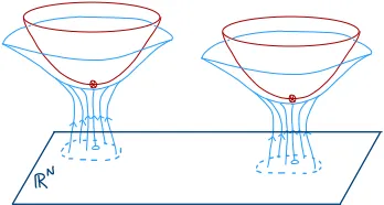
Figure 3. The flow maps point inRN _{to points inMT. The integral overMT equals the one overR}N_{at all} values ofT. AsT increases,MT approaches the combination of thimbles equivalent to the original domain of integration.

3.2 Cheaper jacobians: estimators, Grady-style algorithm

One strategy to deal with the high computational cost of the jacobian is to have a rough estimator of it to be used to generate the Monte Carlo chain. The difference between the estimator and the correct jacobian can be included as a reweigthing factor, as it is done with the phase of the jacobian. We have found two estimators that seem to be useful in (some) of the models we have studied. The first estimator of detJisW1defined by

logW1(ζ)= T

0 dt

N

a=1 e(ia)†

∂2S(φ(t)) ∂φi∂φj e

(a)

j (14)

wheree(a) _{is the (complex) basis formed by the solutions to eq.(11) with positive eigenvalues. The} hessian ∂2S

∂φi∂φj is to be computed along the flow trajectory starting atζwhile the basise

(a)_{is computed} from the hessian at one critical point of a “dominating" thimble. For quadratic actions (free theories), W1=Jand, consequently, it is to be expected thatW1is a good estimator in weakly coupled theories. Experience shows that it is an useful estimator even in theories which, by any measure, are strongly coupled. The second estimatorW2is even simpler to compute:

logW2 = T

0 dttr   ∂

2_S(φ(t))

∂φi∂φj

  =

T

0 dt

N

a=1 e(ia)†

∂2_S(φ(t))

∂φi∂φj e

(a)

j . (15)

W2is the determinant of the matrixW2i jsatisfying the equation

dW2i j

dt =

∂2_S

Figure 3. The flow maps point inRN _{to points inMT. The integral overMT equals the one overR}N _{at all} values ofT. AsT increases,MT approaches the combination of thimbles equivalent to the original domain of integration.

3.2 Cheaper jacobians: estimators, Grady-style algorithm

One strategy to deal with the high computational cost of the jacobian is to have a rough estimator of it to be used to generate the Monte Carlo chain. The difference between the estimator and the correct jacobian can be included as a reweigthing factor, as it is done with the phase of the jacobian. We have found two estimators that seem to be useful in (some) of the models we have studied. The first estimator of detJisW1defined by

logW1(ζ)= T

0 dt

N

a=1 e(ia)†

∂2S(φ(t)) ∂φi∂φj e

(a)

j (14)

wheree(a) _{is the (complex) basis formed by the solutions to eq.(11) with positive eigenvalues. The} hessian ∂2S

∂φi∂φj is to be computed along the flow trajectory starting atζwhile the basise

(a)_{is computed} from the hessian at one critical point of a “dominating" thimble. For quadratic actions (free theories), W1=Jand, consequently, it is to be expected thatW1is a good estimator in weakly coupled theories. Experience shows that it is an useful estimator even in theories which, by any measure, are strongly coupled. The second estimatorW2is even simpler to compute:

logW2= T

0 dttr   ∂

2_S(φ(t))

∂φi∂φj

  = T 0 dt N a=1 e(ia)†

∂2_S(φ(t))

∂φi∂φj e

(a)

j . (15)

W2is the determinant of the matrixW2i jsatisfying the equation

dW2i j

dt =

∂2_S

∂φi∂φkW2k j, (16)

with initial conditionW2i j(t=0)=δi jinstead of

dJi j dt =

∂2S

∂φi∂φkJk j, (17)

satisfied byJ. This suggests thatW2will be a good estimator if Jis nearly real, which agrees with our experience. We emphasize, however, that the use of these estimators does not introduce an uncon-trolled error in the calculation since, when making measurements, the difference between the estimator and the correct jacobian is reweigthed.

A more elegant way of dealing with the cost of the jacobian, which we will call the Grady algo-rithm, is given by a modification of our algorithm in eq.(3.1) that includes a way of bypassing the computation of the jacobian by adapting the Grady algorithm [24,25] originally created to deal with fermion determinants. The main idea [26] is to make a modified proposal that is isotropic in the variableφT(ζ), not inζ, and then correct for that by modifying the accept/reject step. The proposal

probability is given by

P(ζ →ζ)=e−∆ζJ†J∆ζdetJ†J=e−η†ηdetJ†_{J, (18)}

where∆ζ =ζ−ζ,J= J(ζ) is the jacobian matrix andηis a complex vector tangent toMT. The

action ofJon a real vector is the same as evolving the vector by the equations eq.(9). The result is, by construction, a vector tangent toMT:J∆ζ =η. However, flowing an imaginary vector, normal toRN, does not give a complex vector normal toMT. Thus, the proposal with probability above can be found

by picking a random vector from the distribution∼ e−η†_η

, solving iteratively the equationJ∆ζ = η

and then computingη=JRe(∆ζ). The action ofJ−1_{on a complex vector is obtained by flowing the} real and imaginary parts of the vectorseparatelyby theinverseof the flow in eq.(9). The backward flow has to be applied to the real and imaginary parts separately as the flow evolution is not a linear operator (it has an anti-linear part). The accept/reject step proceeds as follows. After a proposalζis chosen, a random real vectorξis chosen with probability distributionp[ξ]=e−ξ†J†JξJ†J√detJ†J by iteratively solvingJ_{ξ=η, whereηis chosen from a gaussian distribution∼e}−η†_η

. The probability of acceptance ofζis given by min(1,e−Se f f[ζ]+Se f f[ζ]). It is easily shown that this procedure satisfies

detailed balance[26].

4 It all comes together in one example:

4.1 The1+1DThirring model

After quite a bit of theoretical discussion it will be good to see how these ideas apply – and how well they fare – in an actual numerical calculations. We choose the 1+1 dimensional Thirring model at finite density (and temperature) as a suitable testing ground. It has the advantage of having less degrees of freedom than a 4-dimensional theory would, while sharing some features with QCD like asymptotic freedom, a formulation where the sign problem appears (only) at finite density and a complex fermion determinant (bosonic sign problems were studied using similar approaches in [12,27–29] ). The model is defined in the continuum by the (euclidean) action

S =

d2_{x[ ¯ψ}α_(∂/+µγ

0+m)ψα₊ g2

2NF

¯

ψα_γ

µψαψ¯βγµψβ], (19)

where the flavor indices take valuesα, β=1, . . . ,NF,µis the chemical potential and the Dirac spinors

¯

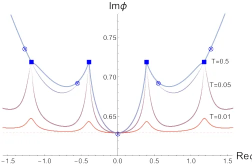
Figure 4. Cross-sectionA0(x)=Reφ+iImφ,A1(x)=0. The thimbles are shown in blue, the critical points are

denoted by a cross and the detD(A)=0 points are the squares. The flow takes point inRN_{to points inM} T. The

integral overMTequals the one overRNat all values ofT. AsT increases,MTapproaches the combination of

thimbles equivalent to the original domain of integration.

[30]; we will describe here the results with Wilson fermions. In that case the discretized action chosen is

S =

x,ν

NF

g2(1−cosAν(x))+

x,y ¯

χα(x)Dxy(A)χα(y), (20)

with

Dxy=δxy−κ

ν=0,1

(1−γν)eiAν(x)+µδν0δx+ν,y+(1+γν)e−iAν(x)−µδν0δx,y+ν

, (21)

Notice we chose to use auxiliary bosonic variables that are periodic so the original manifold of inte-gration of the path integral is (S1₎N_{. This choice makes the model close to gauge theories and avoids}

some of the discussion we had in section2regarding the asymptotic behavior ofMT. The integration

over the fermion fields leads to

S =NF   g12

x,ν

(1−cosAν(x))−log detD(A).

 

, (22)

This action describesNF Dirac fermions in the continuum. Forµ 0 the determinant detD(A) is

not real so this model cannot be simulated by standard Monte Carlo techniques. From here on we

choose NF = 2. In the continuum this model is solvable but, since we will work not too close to

the continuum. The thimble structure of this model is partially understood, specially in the subspace

A0(x) = Reφ+iImφ =constant,A1(x) = 0 where it is similar to the one of the 0+1 dimensional Thirring model [14, 31,32]. There are a number of critical points in the A0(x) = φ,A1(x) = 0 complex plane. There are also points where the action diverges. They arise because the fermion determinant vanishes for some values of theAµfields. They do no imply any singularity in the integral, they actually correspond to zeros of the integrand and the contribution of the fields around them is

Figure 4. Cross-sectionA0(x)=Reφ+iImφ,A1(x)=0. The thimbles are shown in blue, the critical points are

denoted by a cross and the detD(A)=0 points are the squares. The flow takes point inRN_{to points inM} T. The

integral overMTequals the one overRNat all values ofT. AsT increases,MTapproaches the combination of

thimbles equivalent to the original domain of integration.

[30]; we will describe here the results with Wilson fermions. In that case the discretized action chosen is

S =

x,ν

NF

g2(1−cosAν(x))+

x,y ¯

χα(x)Dxy(A)χα(y), (20)

with

Dxy=δxy−κ

ν=0,1

(1−γν)eiAν(x)+µδν0δx+ν,y+(1+γν)e−iAν(x)−µδν0δx,y+ν

, (21)

Notice we chose to use auxiliary bosonic variables that are periodic so the original manifold of inte-gration of the path integral is (S1₎N_{. This choice makes the model close to gauge theories and avoids}

some of the discussion we had in section2regarding the asymptotic behavior ofMT. The integration

over the fermion fields leads to

S =NF   g12

x,ν

(1−cosAν(x))−log detD(A).

 

, (22)

This action describesNF Dirac fermions in the continuum. Forµ 0 the determinant detD(A) is

not real so this model cannot be simulated by standard Monte Carlo techniques. From here on we

choose NF = 2. In the continuum this model is solvable but, since we will work not too close to

the continuum. The thimble structure of this model is partially understood, specially in the subspace

A0(x) =Reφ+iImφ =constant,A1(x) =0 where it is similar to the one of the 0+1 dimensional Thirring model [14, 31,32]. There are a number of critical points in the A0(x) = φ,A1(x) = 0 complex plane. There are also points where the action diverges. They arise because the fermion determinant vanishes for some values of theAµfields. They do no imply any singularity in the integral, they actually correspond to zeros of the integrand and the contribution of the fields around them is

suppressed. Since the action approachesSR → ∞there, they are attractors of the anti-holomorphic

Figure 5. Fermion density versus chemical potential (left panel) and average sign versus chemical potential (right panel).

flow. The picture that emerges is that these singularities of the action arise at the border of the thimbles and different thimbles approach these singularities from different directions. The manifold defined by

detD(A) = 0 has 2N−2 (real) dimensions. Two manifolds, each with dimensions N, generically

meet only at isolated points with dimensions 0. But thimbles are tangent to the anti-holomorphic flow that “seeks" points with divergent action so they end up meeting at a larger dimensional space. This structure is generic to models with fermions and it is depicted on fig.4.

Let us consider some specific values of the parameters for illustrative purposes. Withm=₋0.25,

g =1.0 we find, by performing standard Monte Carlo at zero density on a 10×10 lattice, a fermion

massamf =0.30(1) and a bosonic mass (for the state generated in the continuum by ¯ψaγ5τ3abψb) of amb = 0.44(1). Since mb << 2mf these parameters correspond to a strongly coupled model. An

attempt at simulating this model with usual techniques, namely, an integration over (S1₎N_{reveals that}

there is a terrible sign problem for all chemical potentials largermf. In fig.5we show the average sign

(right panel) and the fermions density (left panel). It is evident that, even on this small lattice, there is a severe sign problem.

The critical point with the smallest action is the one nearest to (S1₎N_atφ=φ

c=purely imaginary

and, at least at weak coupling, is expected to dominate the path integral. The tangent plane to the thimble atφcis purely real. If we take the domain of integration to be this tangent plane we expect

the sign problem to improve as compared to the one on (S1₎N _{since the action, and therefore its}

imaginary part, varies only quadratically with the deviation from the critical point. In other words, the tangent plane is a good approximation to the thimble for points near the critical point. Since the phasee−iSI is fixed on the thimble, we expect it to vary little on the tangent plane. This expectation is supported by actual calculations shown in fig.5. Notice that calculations on the tangent plane are just as computationally cheap as the usual integration over real variables. Still, for values of the chemical potential high enough (µ > 3mf) the sign problem returns, even in these modest lattice sizes. We

now use the algorithm described in section3except that we start the flow not from real values of the fieldAµ(x) but from theA0(x) =φc,A1(x)=0 plane in order to take advantage of the improvement

a

N

a

N

Figure 6. Contour in the complext-plane used in the Schwinger-Keldysh formalism.

flow times is shown in fig.4. As discussed above, the higher the value ofT the closerMT is to the

(correct combination of) thimbles. The integrations over each one of these manifoldsMT give the

same result but at different computational cost as the sign problem is much milder at largerT. This can be seen on fig.5. The average sign becomes much larger already atT =0.4, almost completely solving the sign problem and leading to the results on the left panel of5. There is a price to pay, however, ifTis too large. The regions ofMTcontributing significantly to the integral are mapped by

regions of (S1₎N_{that are well separated by barriers of low probability∼e}−SR. This situation is hard to

be dealt with by any Monte Carlo calculation (although “tempered" algorithms have been used to deal with it [22,23]). If not extra care is taken (and the computational resources spent), the Monte Carlo chain becomes trapped in one of the modes of the distribution and only the region ofMTclose to one

of the thimbles is properly sampled. In cases where the contribution of the other thimbles is sizable (given the statistical uncertainty of the measurements), the final result is erroneous. On the other hand the trapping due to excessive flow can be used to separate the contribution of different thimbles to a given observable. In [21], the 0+1 dimensional Thirring model was studied and it was shown that the trapped calculation, sampling only one thimble, gives results that differ by small but statistically significant, amounts from the exact analytic result (the single thimble calculation discussed in [33] also agrees with our trapped calculation.). The approach to the thermodynamics and continuum limits in this model does not seem to bring any extra difficulties in this model [21]. In particular, the plateau structure on observables due to shell effects in a finite volume are very visiby and correctly described by the calculations. As pointed out in [15], this structure is washed out if the contribution of only one thimble is taken into account.

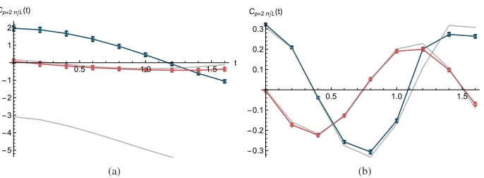
4.2 Real Time Dynamics

a

Nt

a

N

Figure 6. Contour in the complext-plane used in the Schwinger-Keldysh formalism.

flow times is shown in fig.4. As discussed above, the higher the value ofT the closerMT is to the

(correct combination of) thimbles. The integrations over each one of these manifoldsMT give the

same result but at different computational cost as the sign problem is much milder at largerT. This can be seen on fig.5. The average sign becomes much larger already atT =0.4, almost completely solving the sign problem and leading to the results on the left panel of5. There is a price to pay, however, ifTis too large. The regions ofMT contributing significantly to the integral are mapped by

regions of (S1₎N_{that are well separated by barriers of low probability∼e}−SR. This situation is hard to

be dealt with by any Monte Carlo calculation (although “tempered" algorithms have been used to deal with it [22,23]). If not extra care is taken (and the computational resources spent), the Monte Carlo chain becomes trapped in one of the modes of the distribution and only the region ofMTclose to one

of the thimbles is properly sampled. In cases where the contribution of the other thimbles is sizable (given the statistical uncertainty of the measurements), the final result is erroneous. On the other hand the trapping due to excessive flow can be used to separate the contribution of different thimbles to a given observable. In [21], the 0+1 dimensional Thirring model was studied and it was shown that the trapped calculation, sampling only one thimble, gives results that differ by small but statistically significant, amounts from the exact analytic result (the single thimble calculation discussed in [33] also agrees with our trapped calculation.). The approach to the thermodynamics and continuum limits in this model does not seem to bring any extra difficulties in this model [21]. In particular, the plateau structure on observables due to shell effects in a finite volume are very visiby and correctly described by the calculations. As pointed out in [15], this structure is washed out if the contribution of only one thimble is taken into account.

4.2 Real Time Dynamics

As is well known, a number of observables like particle masses and matrix elements, can be extracted from the imaginary time correlators. Other observables like transport coefficients can be found only from real time correlators. While in thermal equilibrium the real time correlators can be, in principle, obtained from the knowledge of the imaginary time ones, the process requires an analytic continua-tion from the discrete, imaginary values of energy available in the Matsubara formalism to continuous real energies. Although the analytic continuation is possible (and unique), the analytic continuation is numerically unstable and the statistical uncertainty of a Monte Carlo calculations makes it nearly im-possible in practice. An alternative approach would be a direct calculation in real time. A framework for calculations of thermal averages in real time exists, the so-called Schwinger-Keldysh formalism

[34, 35]. It has been almost exclusively used in conjunction with weak coupling expansions (the exceptions we are aware of are the complex Langevin studies in [36–39] ).

Consider a system described initially by a density matrix of the formρ = e−βH/Z 5 and whose

evolution in time is governed by the hamiltonianH. We will be interested in observables of the form O1(t1)O2(t2) = tr (ρO1(t1)O2(t2)). In the case H = H this is an equilibrium correlation function and it depends on the differencet1−t2. Fully non-equilibrium situations can be dealt with the same formalism but, for now, we will restrict ourselves to the equilibrium case.

Expectation value of observables are given by:

O(t) = tr (ρO(t))=trρ(0)U(t,0)OU†_{(t,0) (23)} = tr (U(−iβ,₋iβ/2)U(−iβ/2,T−iβ/2)U(T −iβ/2,T)U(T,t)OU(t,0)) (24)

whereU(t,t) = e−iH(t−t) andT is an arbitrary timeT > t. The case of 2-point functions or more

is dealt with similarly. This expression describes the propagation from 0 tot, then toT, down to T−iβ/2, then backwards to−iβ/2 and down the along the imaginary direction to−iβ. It has a path integral representation in terms of an action defined on a time contour in the complextplane depicted in fig.66_:

O(t)=

Dφe−SS K[φ]_O

Dφe−SS K[φ] . (25)

The contour actionScis purely imaginary along the part of the contour lying on the real axis. The

discretization we used was:

SS K[φ]=

t,n ata

₍

φt+1,n−φt,n)2

2a2

t

+1 2

₍

φt+1,n+1−φt+1,n)2

2a2 +

(φt,n+1−φt,n)2

2a2

+ m 2 2

φ2_t,n+φ2t+1,n

2 +

λ

4!

φ4_t+1,n+φ4_t,n

2  

 (26)

wheretandnindexes the lattice along the time and spatial directions,ais the spatial lattice spacing andatis the time lattice spacing:

at = ia, for 0≤t<Nt, at = a, for Nt≤t<Nt+Nβ/2,

at = −ia, for Nt+Nβ/2≤t<2Nt+Nβ/2,

at = a, for 2Nt+Nβ/2≤t<2Nt+Nβ, (27)

andNt,Nβare the number of lattice points on the real and imaginary axis, respectively.

The integral in eq.(25) has “perfect" sign problem: the average sign is not small but strictly zero, as can be seen by considering the variation of the contour action when the value of the field on a real value oftis considered. The real part of the action is not changed by this variation and there is no damping of the Boltzmann factor asφ(t) is varied.

The application of the generalized thimble method to real time problems faces some extra diffi cul-ties. Consider, for instance, a 1+1 dimensionalφ4theory [26]. The first problem is that the tangent plane to the critical pointφc=0 is not real and, in some directions in field space, points towards the

imaginary direction. Therefore, the tangent space is likely not in the same homology class asRNand 5_{There is no loss of generality assuming this form ofρ.}

6_{There is a certain latitude in the choice of this contour. All that is required is that it starts att=0, ends att=−iβa passes}