Ozone Variability over Egypt

1

Ozone Variability over Egypt

Ayman Badawy 1,*_{, Heshmat Abdel Basset} 2,* _{and Mohamed Eid} 2

1 _{Egyption Meteorological Authority, El Khalifa El Maamoun St., Kobry El Koba, Cairo, P.O.BOX} 11784, Egypt;

2 _{Department of Astronomy and Meteorology, Faculty of Science, Al-Azhar University, 1 Al Mokhaym} Al Daem, Gameat Al Azhar, Nasr City, Cairo, Egypt.

* Correspondence: [email protected] (A.B.); [email protected] (H.A.B.)

Abstract: The variability of ozone over Egypt has been studied in this work. Higher values of coefficient of variation (COV) at eight stations occur at winter while lowest values occur at summer. The COV is function of latitude in annual, winter and spring where it decreases gradually from the north to south of Egypt. The trend analysis of ozone over the eight stations indicates negative trends over northern stations for both annual and seasonal time series with the greatest one at winter. The horizontal distribution of ozone trend values is negative over all Egypt in winter while it positive over middle and south Egypt in the other seasons. The long-term variability of the behavior of the annual ozone shows positive trend values in ozone are the dominant features during the period 1979- 1989 at the most stations. Negative trend values in ozone are the dominant features during the period 1990- 2014 at all stations. The Mann–Kendall test confirms that there is an abrupt change towards decreasing of ozone occurs in 1981, 1984, 2012, 1999, 2000, 1998 and 2010, while a change towards increasing of ozone appears in 2006, 2014, 1993 and 1989.

Keywords: total ozone; seasonal variation; analysis trend; homogeneity; abrupt change

1. Introduction

2

prevents most harmful UV radiation from reaching the biosphere, Due to this high energy, UV-B radiation can have several harmful impacts on human beings ( DNA damage, skin cancers, corneal damage, cataracts, immune suppression, aging of the skin, and erythema), on ecosystems, and on materials ( UNEP, 1998, 2003). So we have to protect ozone layer from depletion, the study variation and trend of total column ozone is very important to detected its behavior many early studies has performed to the trend of ozone depletion, one of the ways to study the time series behavior is Abrupt change, which can be generally defined as occurring when some part of the climate system passes a threshold or tipping point resulting in a rapid change that produces a new state lasting decades or longer (Alley et al., 2003). In this case “rapid” refers to timelines of a few years to decades.

3

2. Data

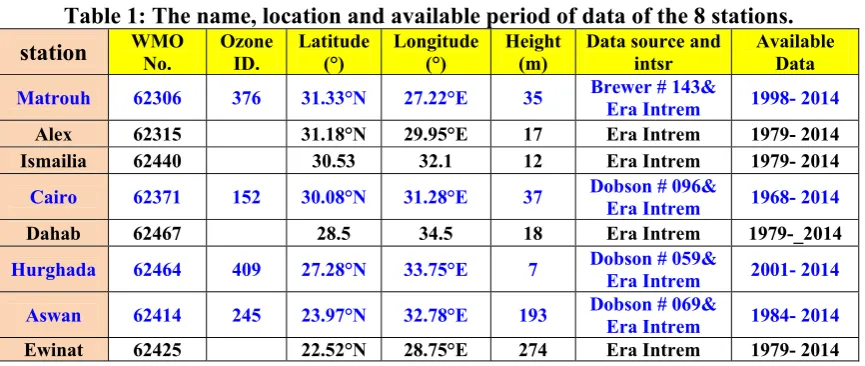
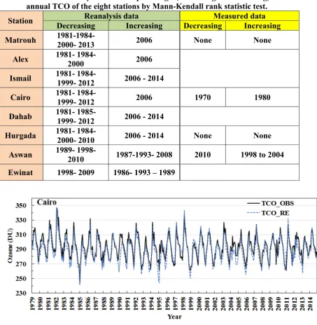
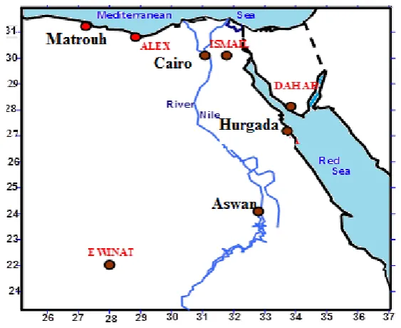
In Egypt there are four stations providing ground-based total ozone measurements. Table 1 illustrates the name, location, the instrument type used to measure total ozone and the period of measurements for each station. Occasionally, there are missing data (about 1% of the total data) which need to be dealt with in some fashion for calculation of the climatology. Linear interpolation is used to estimate missing values in order to make the time series complete, which enables a computation of monthly and yearly means and a time series analysis of the daily data. We also extract another four time series of TCO for the previous four stations from reanalysis ERA- Intrem total column ozone data (http://apps.ecmwf.int/datasets/data/interim-full-moda). To cover and represent the different regions of Egypt we also obtain the time series of TCO for the stations Alex (29o_{E, 31}o_{N), Ismail (32}o_{E, 30}o_{N), Dahab (34}o_{E, 28}o_{N) and Ewinat (28}o_{E, 22}o_{N). The} comparison between TCO of ground based station and its corresponding reanalysis data has been verified over Cairo and represented in Fig. 1. It is found that there is a very good agreement between observed and reanalysis data, where the correlation coefficient is 0.91 and the root mean square error is 6.1, this good agreement allowing us to use this data in our study. Figure 2 shows the study area and the location of eight stations, four of them are the ground-based stations while the other four stations we used the reanalysis ozone data. The reanalysis daily and monthly data for total amount of ozone and other meteorological parameters are obtained from (http://apps.ecmwf.int/datasets/data/interim-full-moda). ERA-Interim reanalysis data is the latest global atmospheric reanalysis data set of the European Center Weather Forecast (ECMWF) with period from 1979 till 2014 with resolution 1o_x1o _{is used for obtain total column ozone from meteorological} parameters.

3. Methodology

4

calculated using the following relation (Mitchell et al. 1966):

( )

1

1 2 2

2 _      ₋

=





S

Where the summations range over the n values of the Series, Σi in the subperiod K. The estimated ratio between the maximum and minimum values

(

S

/

S

)

A coefficient of variation (COV) for each individual station has been determined as follows:

μ / *

100 SD

COV = (2) Where, SD is the standard deviation and

μ

Different methods have been applied to study the trend and fluctuations of ozone over the studied area. These methods are; (a) Linear regression by using Least Square method (Panofsky and Brier ,1963), (b) Gaussian low-pass filter (Mitchell et al 1966), (c) Binomial low-pass filter (Mitchell et al. ,1966 and Tyson et al.,1975). Also the non-parametric Mann-Kendall (M-K) rank correlation test (Sneyers, 1990; Schonwiese and Rapp, 1997; Hasanean, 2004) has been used to detect any possible trend in ozone series, and to test whether or not such trends are statistically significant. To visualize the decadal and inter-decadal fluctuations or “persistence” in the behavior of the KSA ozone, cumulative seasonal means method is used (Pavia and Graef 2002). The advantage of this is to reveal time varying structures in time series. The cumulative seasonal means time series can be defined as;



, j =1,2,..., N. (3) Where,

x

N

Abrupt change procedur:

5

detecting the beginning of any change in a time series (Goossens and Berger 1986). The intersection between the two resulting trend lines in the region ±1.96 of the standardized statistic, at the 5 % significant level, is considered to be an evidence of an abrupt change in the time series. Estimation of MK rank statistic is done by considering only the relative values of all the terms in the time series X_i under analysis and replacing the X_i values with their ranksY_i, arranged in increasing order. For each elementY_i, the number n_i of elements Y_j preceding it, i.e. (ij) is calculated such thatY_iY_j. The statistical test T_i is then given by the following formula:

i

i n n n

T = ₁+ ₂+...+ (4)

This sum is standardized to a normal distribution by

[

]

)

(T_i T_i ET_i T_i

u = − (5) Where the mean E(T_i) and variance var(T_i) are defined as

, 4 ) 1 ( ) (T =ii−

E _i 72 ) 5 2 )( 1 ( )

var(T_i =ii− i+ (6)

A significant trend at the threshold

α

_α

α

). (

1= p u ui

α (7)

If the values of u(T_i) are significant, then they can be considered whether the trend

is increasing or decreasing, by looking at how u(T_i) itself increases or decreases. However, when a series shows a significant trend, it is necessary to locate the start of the abrupt change by means of a sequential analysis. In this case, the analysis is performed with the same time series but with reversed sequence. To identify an abrupt change in the time series, this analysis is performed with the same SAT time series but with the reverse sequence, i.e., number /

i

n of Y_j terms for each Y_i term, such that Y_iY_j withi jwill be i

i

i Y n

n/ = −1− (8)

So that, i/ =(N+1)−i (9)

6

absence of any trend in the series, the graphical representation of u and u′ in terms of i generally gives curves, which overlap several times.

Mann- Whitney test for step trend

Given the data vectorX=(x₁,x₂,...,x_n), partitionX so that Y=(x₁,x₂,...,x_n1)and )

..., ... , ,

(x_n11 x_{n1 2} x_{n1 n2}

Z= _{+ + +} . The Manne Whitney test statistic is given as:

[

]

2 / ) 1 ( )

( _{1 1 2 1 2 1 2} 1/2

1 1 + +         + + − =



in which r(x_t)is the rank of the observations. The null hypothesis H0 is accepted if 2

/ 1 2

/

1−α ≤ ≤ −α

−Z Z_c Z , where ±Z_1−α/2 are the 1−α/2 quantiles of the standard normal distribution corresponding to the given significance level α for the test.

4. Results

4.1 Homogenity of the data

Study of the data homogeneity is important in climatology. Homogeneity is established differently in different climatic elements. The values of climatic elements could be the method of estimating daily and monthly averages. Artificial lakes and reservoirs and other man-made changes of local environment produce sources of inhomogeneity in historical record of climatic data.

Homogeneity of the total column ozone (TCO) of the annual and seasonal time series over Egypt stations has been detected by means of Bartlet test (described in section 3). Table 2 shows Bartlet test (short-cut) result for annual and seasonal ozone of land based stations and reanalysis data respectively. The mean annual and seasonal of TCO seems to be homogeneous for all stations regarding the ratio (S_max2 /S_min2 ) Bartlet test with 95% significance as shown in (Mitchell et al., 1966).

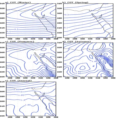
4.2 Coefficient of variation (COV)

7

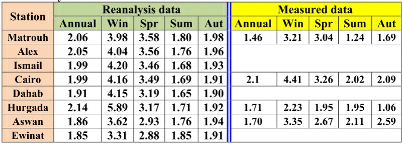
The COV of annual, winter, spring, summer and autumn of TCO of the reanalysis (8 stations) and measured (4 stations) data is displayed in Table 3. The higher values of COV at all stations occur at winter while the lowest values of COV occur at autumn. The COV of spring at all stations are greater than those in summer and annual values. The COV in annual and winter decreases gradually from the northen station to the southern station. So it can be said that the COV is a function of latitude in winter and annual values. The maximum value of COV in spring and autumn for the eight stations occurs at Matrouh, it reaches 3.58 and 1.98 respectively. Also as in winter, the values of COV in spring decrease gradually from the northern station to the southern station. In summer season the behaviour of COV at our stations is different from that in winter, spring and autumn seasons, these results are more obvious in Figure 3. Figure 3 illustrates the horizontal distribution of COV for the annual and seasonal values of TCO. It is clear that the values of COV of winter, spring and annual decreases gradually from north to south of Egypt. The patterns of COV for summer and autumn are different from winter and spring, where we found that the summer values of COV decreases from west to east, it may be affected by the west ward oscillation of the Indian monsoon low. The lowest values of COV of autumn appears at the middle of south Egypt and also over the Red Sea, it may be associated with the northward oscillation of the inverted V-shep trough of Sudan low. The high variability over north Egypt in winter and spring is associated with the traveling main and secondary Mediterranean cyclones.

4.3 Trend analysis

The annual ozone time series for the eight stations under study have been investigated to determine their trends. The studies of trends have been performed by means of both a simple and sophisticated tools. These methods are: 1) Least square method of first order (linear regression), 2) Moving filters by using Gaussian low- pass filter and binomial low- pass filter and 3) Mann-Kendall rank statistical test. Discussion of the important aspects of the long-term variations and trends are given below for annual ozone time series.

4.3.1 Trend by least square method

8

seasonal ozone of Egypt stations. It showed that there is a positive trend of annual and seasonal ozone at four ground-based stations. It is clear that the only negative trend occurs only in winter over Cairo (-0.15 DU/year), also the minimum annual trend value occurs at Cairo (0.03DU/year). With respect to the reanalysis TCO time series of the eight station, it is found that the maximum annual and seasonal trends occurs at Hurgada and Matrouh, it may be due to the location of these two costal stations ( Beig et al. 2007).

The trend of the reanalysis TCO time series of the eight stations is positive for the autumn season. Also, the trend of the southern three stations (Hurgada, Aswan and Ewinat) is positive for the annual and seasonal TCO time series.

4.3.2 Fluctuation of annual Ozone

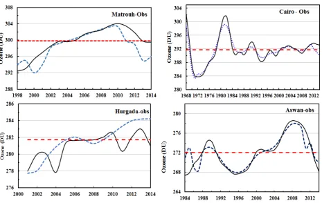
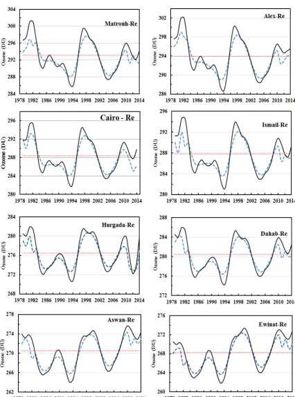
Trends of annual ozone of the concerned stations by means of Gaussian and binomial low- pass filter (dotted curve, thin curve) has been investigated for ground based (observed) and reanalysis data (Figures 4 and 5 ).

Figure 4 illustrate the results obtained from the two methods for the observed values of TCO. Careful examination of the obtained results shows that during the period 2004 to 2013 an obvious increase of TCO occurred in Matrouh and Aswan, the increase in mean annual TCO reached to 4 DU. A pronounced decrease of TCO at Matrouh appears from 1998 to 2002, after that TCO have its average value until 2005. From 2006 to 2013 an obvious increase of TCO occurs at Matrouh, the maximum increase (4 DU) appears at the years 2009 and 2010. For Cairo station a decrease of TCO has been found from 1969 to 1977 with a maximum reached to 4 DU during 1970 to 1973, followed by an obvious increase of TCO from 1978 to 1984. During the period from 1985 to 2014, the values of TCO fluctuate around the mean. For Hurgada a decrease of TCO is found from the beginning until 2005, this period followed by a persistence of TCO around the mean until 2009. During the last period TCO fluctuate around its mean with considered amplitude. The behavior of TCO time series in Aswan can be divides into two obvious periods, the first one is from 1990 to 2000 is dominated by a decrease of TCO. The second period (2004- 2012) is characterized by a pronounced increase of TCO.

9

behavior of each time series can be divided into five periods, the first one is from 1979 to 1983 and characterized by increase of TCO with maximum at 1980, this period followed by a respectively long period of decreasing of TCO which extended from 1982 to 1995 with maximum decrease at 1994. The third period (1995- 2002) is dominated by increase of TCO with maximum at 1997. An obvious decrease of TCO occurs during the fourth period (2002- 2008) with maximum decrease at 2004. The last period (2008- 2014) is characterized by increase of TCO except for Hurgada station. Although there is a considerable difference between the record length of the time series of the observed and reanalysis data, there is a high consistence between the results. As examples, the period from 2001 to 2005 represent a period of decrease of TCO in Hurgada in observed and reanalysis data, while the period 2007 to 2014 represent a period of increase of TCO. Also, there is a high consistence between the periods of increase and decrease in observed and reanalysis data of Cairo especially for the increase period 1979- 1983. Two periods of high consistence between observed and reanalysis data appears at Aswan, the first is from 2006 to 2012 while the second is from 1991 to 2000.

4.3.3 Mann-Kendall rank statistical test

1979-10

2014. It shows that in winter the negative trend values appears north of latitude 22o _{N and} in spring north of latitude 28o _{N, while in summer and autumn it appears north of 30}o _N.

4.4 Cumulative annual means

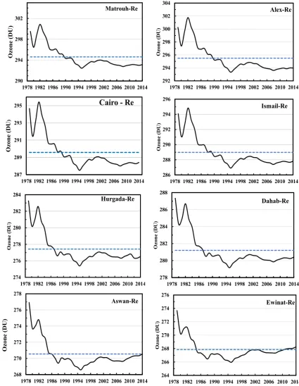
To visualize the decadal and inter-decadal fluctuations or “persistence” in the behavior of the Egypt ozone, cumulative annual means method is used (Pavia and Graef 2002). The advantage of this is its ability to reveal time varying structures in time series. In this section, the long- term variability of the behavior of the annual ozone is analyzed with regard to the time variations of annual ozone. Cumulative annual means will be used to visualize the decadal and inter-decadal fluctuations in the behavior of the annual ozone, because they advantageously reveal time varying structures in time-series, which are not readily recognizable in raw data. Moreover, the cumulative means have a smoothing effect, similar to low-pass filters (Lozowski et al., 1989). Persistent phases of alternating increase or decrease of the ozone, which vary in length, are recognizable in the time series of the annual ozone.

Figure 7 illustrate the cumulative annual mean (CAM) time series and the averaged CAM of the measured annual values of ozone of the stations Cairo, Matrouh, Hurgada and Aswan. Results from Cairo station show that CAM time series can be divided into three periods. The first period (1968-1971) illustrates a positive trend, the second period shows a negative trend, while the last period (1981- 2014) shows a fluctuation of the trend around the CAM average. The cumulative annual means for Matrouh and Hurgda have the same behavior throughout their observational period. They show a negative trend in TCO during the first period (1998-2005) followed by a continuous positive trend until 2014. The maximum average CAM for these stations occurs in Matrouh (297.2 DU). The cumulative annual mean for Aswan throughout its observational period shows a negative ozone trend during the first period (1984- 1989) followed by a positive trend until 1994. A negative trend is detected at Aswan for the period 1994- 2004 followed by a positive trend until 2014. The average CAM of this station is about 271 DU.

11

positive trend values in ozone are the dominant features during the period from 1979 to 1988 at the northern stations (Matrouh, Alex, Ismail, and Cairo), while from 1979 to 1984 at the middle and southern stations (Dahab, Hurgada, Aswan and Ewinat). Negative trend values in ozone are the dominant features during the period 1990- 2014 at the eight stations.

4.5 Abrupt change analysis

12

(Ismail, Dahab, Hurgada). A trend toward decreasing around 2012 occurs in Ismail, Cairo, and Dahab. From the above results one can conclude that a change towards decreasing TOC is obtained in 1981, 1984, 2012, 1999, 2000, 1998 and 2010 and a change towards increasing TOC is obtained in 2006, 2014, 1993 and 1989 (Table 6).

The results of the Manne Whitney test for abrupt change of the time series of TOC for the four ground based stations are illustrated in Figure 11. Figure 11a shows the departure curves of the ozone in Matrouh, departure is the deference of climate variables for 17 years. The test detected abrupt change in the ozone time series of Matrouh around 2006 at the 0.01 significance level. Also there are two obvious periods in the study area for the past 17 years, the first one is the decrease period of 1989-2005, in which the negative departures account for more than 47%, and the abnormal decrease years are 1998, 1999, 2002 and 2004 respectively. The second one is the increase period of 2007-2014, in which the mean ozone is 2.48 DU higher than the average of the whole period. In the increase period, the positive departures account for more than 52%, in which the highest ozone for 17 year and the ozone in 2009 is 6.76 DU higher than that of the whole period. The Manne Whitney test detected two abrupt changes in the ozone time series of

Cairo the first one is around 1979 at the 0.05 significance level while the second one is around 1993 at the 0.08 significance level, Figure 11b shows the departure curves of the ozone in Cairo station. It is shown that the departure curve fluctuates significantly, with the characteristics of two decreasing and one increasing abrupt changes since the 1968s. The period of more ozone, 1980-1992, in which the mean ozone is 2.9 DU more than that of the whole period. The first period of less ozone from 1968 to 1977, in which the mean ozone is 4.49 DU less than that of the whole period. The second period of less ozone is from 1994 to 2014, in which the mean ozone is 0.29 DU less than that of the whole period.

The Manne Whitney test detected abrupt change in the ozone time series of

13

2010 to 2014, in which the ozone is 1.83 DU higher than that of the whole period. The Manne Whitney test detected two abrupt changes in the ozone time series of Aswan the first one is around 2000 at the 0.004 significance level while the second one is around 2012 at the 0.176 significance level, Figure 11d shows the departure curves of the ozone in Aswan station. It is shown that the departure curve fluctuates significantly, with the characteristics of two decreasing and one increasing abrupt changes since the 1984s. The period of more ozone, 2001-2011, in which the mean ozone is 3.5 DU more than that of the whole period. The first period of less ozone from 1984 to 1999, in which the mean ozone is 2.36 DU less than that of the whole period. The second period of less ozone is from 2013 to 2014, in which the mean ozone is 2.48 DU less than that of the whole period.

5. Summary and conclusions

14

values in ozone are the dominant features during the period 1990- 2014 at all stations. The Mann–Kendall test confirms that there is an abrupt change towards decreasing of ozone occurs in 1981, 1984, 2012, 1999, 2000, 1998 and 2010, while a change towards increasing of ozone appears in 2006, 2014, 1993 and 1989.

The study of the Manne Whitney test for abrupt change of the time series of TOC for the four ground based stations confirms that there is abrupt change in the ozone time series of Matrouh around 2006 at the 0.01 significance level. And there are two obvious periods; the first one is the decrease period of 1989-2005 in which the abnormal decrease years are 1998, 1999, 2002 and 2004 respectively. The second one is the increase period of 2007-2014, in which the mean ozone is 2.48 DU higher than the average of the whole period. The Manne Whitney test detected two abrupt changes in the ozone time series of Cairo the first one is around 1979 at the 0.05 significance level while the second one is around 1993 at the 0.08 significance level. The period of more ozone, 1980-1992, in which the mean ozone is 2.9 DU more than that of the whole period. The first period of less ozone from 1968 to 1977, in which the mean ozone is 4.49 DU less than that of the whole period.

References

1- Alley, R.B., et al., 2003: Abrupt climate change. Science, 299(5615), 2005–2010. 2- Atkinson, R.J., Matthew, W.A., Newman, P.A. and Plumb, R.A. 1989: Evidence

of the midlatitude impact of Antarctic ozone depletion, Nature, 340, 290.

3- Beig, Gufran, Singh, Vikas. 2007 Trends in tropical tropospheric column ozone from satellite data and MOZART model, GEOPHYSICAL RESEARCH LETTERS, , Volume 34, Issue 17 :DOI: 10.1029/2007GL030460.

4- Bodeker, G.E., J.C. Scott, K. Kreher and R.L. McKenzie, 2001. Global ozone trends in potential vorticity coordinates using TOMS and GOME intercompared against the Dobson network. Journal of Geophysical Research, 106(D19):23029– 23042.

15

6- Bojkov, R.D. and V.F. Fioletov, 1995: Estimating the global ozone charateristics during the last 30 years. J. Geophys. Res., 100, 16537–16551.

7- Bromwich, D. H., and R. L. Fogt, 2004: Strong trends in the skill of the ERA-40 and NCEP/NCAR Reanalyses in the high and middle latitudes of the Southern Hemisphere, 1958-2001. J. Climate, 17, 4603-4619.

8- C.D.Schonwiese and J.Rapp. Kluwer 1990: Climate trend atlas of Europe based on observations 1891-1990, RmetS,Vol 18, Issue 5 , 580–581

9- David W. Fahey and Michaela I. Hegglin Coordinating Lead Authors Twenty Questions and Answers About the Ozone Layer: 2014 Update

10- De la Casinière A., 2003. Le rayonnement solaire dans l'environnement terrestre. Éditions Publibook, Paris, p 264.

11- E. P. Lozowski, R. B. Charlton, C. D. Nguyen, J. D. Wilson. 1989 . The Use of Cumulative Monthly Mean Temperature Anomalies in the Analysis of Local Interannual Climate Variability Journal of Climate 2(9):1059-1068.

12- Farman J. C., B. G. Gardiner,and J. D. Shanklin, 1985. Large losses of total ozone in Antarctica reveal seasonal Cl0x/NOx interaction. Nature 315, 207-210.

13-Fioletov V. E. and T. G. Shepherd, 2005. Summertime total ozone variations over middle and polar latitudes. Geophys Res. Lett. 32, L04807, doi:10.1029/2004GL022080.

14- Fioletov V. E., G. E. Bodeker, A. J. Miller, R. D. McPeters and R. Stolarski, 2002. Global and zonal total ozone variations estimated from ground-based and satellitemeasurements:1964-2000.J.Geophys.Res.107, .

15- Flohn. H., 1986a. Singular events and catastrophes now and in climatic history, Naturwissenschaften, 73: 136-149

16

17- H.M.Hasanean 2004:Variability of the North Atlantic subtropical high and associations with tropical sea-surface temperature, RmetS.Volume 24, Issue 8,945–957

18- Jeffery C Rogers , 1985, Atmospheric Circulation Changes Associated with the Warming over the Northern North Atlantic in the 1920s, Journal of Applied Meteorology 24(12):1303-1310.

19- Kevin E. Trenberth and Dennis J. Shea,2005, Relationships between precipitation and surface temperature, GEOPHYSICAL RESEARCH LETTERS, VOL. 32, L14703

20- Krzyscin, J.W. 1994: ‘Changes in ozone trends over the northern hemisphere middle latitudes during the period 1970–1990’, Theor. . Appl. Climatol. 49, l 7.

21- LENNART BENGTSSON, VLADIMIRA. SEMENOV, OLAM.

JOHANNESSEN, 2004, The Early Twentieth-Century Warming in the Arctic—A Possible Mechanism, Journal of Climate, 17, 4045–4057.

22- Miller, J.R., G.L. Russell, and G. Caliri, 1994: Continental-scale river flow in climate models.J.Climate,7,914-928.

23- Mitchell JM Jr, Dzerdzeevskii B, Flohn H, Hofmeyr WL, Lamb HH, Rao KN, Wallén CC (1966) Climatic Change. WMO Technica l Note No 79, World Meteorological Organization, Geneva, p 79.

24- Molina M. J. and F. S. Rowland, 1974. Stratospheric sink for chlorofluoromethanes: chlorine atom-catalyzed destruction of ozone. Nature 249,810-812.

25- Newchurch M. J., E.-S. Yang, D. M. Cunnold, G. C. Reinsel, J. M. Zawodny and J. M. Russell III, 2003. Evidence for slowdown in stratospheric ozone loss: First stage of ozone recovery. J. Geophys. Res. 108, doi:10.1029/2003JD003471. 26- Panofsky, H. A., and G. W. Brier, 1963:Some Applications of Statistics to

meteorology . Penn State University,224 pp.

27- Pavia EG, Graef F. 2002.: The recent rainfall climatology of the Mediterranean Californias. Journal of Climate15: 2697–2701.

17

groundbased and TOMS total ozone data through 1991. J. Geophys. Res., 99, 5449–5464.

29- SHI Xiaohui,XU Xiangde,XIE Li'an , 2007: Reliability Analyses of Anomalies of NCEP/NCAR Reanalyzed Wind Speed and Surface Air Temperature in Climate Change Research in China, Journal of Meteorological Research 2007, Vol. 21

Issue (3): 320-333

30- Sneyers, R. (1990): On the Statistical Analysis of Series of Observations. Technical Note 143, WMO-No. 415, Geneva, 192 p.

31- Stolarski R. S. and S. M. Frith, 2006. Search for evidence of trend slow-down in the long-term TOMS/ SBUV total ozone data record: the importance of instrument drift uncertainty. Atmos. Chem. Phys. 6, 4057-4065.

32- Stolarski, R.S., Bloomfield, P., McPeters, R.D. and Herman, J.R. 1991: ’Total ozone trends deduced from Nimbus 7 TOMS data’, Geophys. Res. Lett. 18, 1015. 33- Stolarski, R.S., Bojkov, R., Bishop, L., Zerefos, C., Stachelm, J. and Zaaurodny,

J. 1992: Measured trends in stratospheric ozone, Science, 256, 342–349

34- Stolarski, R.S., Krueger, A.J., Schoeberl, M.R., McPeters, R.D., Newman, P.A. and Alpert, J.C., 1986: Nimbus 7 satellite measurements of the springtime Antarctic ozone decrease. Nature, 322, 808–811.

35- Trenberth, K.E., 1990: Recent observed interdecadal climate changes in the northern Hemisphere. Bull. Am. Meteorol. Soc., 71, 988–993.

36- UNEP, 1998. Environmental Effects of Ozone Depletion. United Nations Environment Programme.

37- UNEP, 2003. Environmental Effects of Ozone. Depletion: 2002 Assessment. Photochemistry and Photobiology, 2:1–72. United Nations Environment Programme.

38- W. Chehade, M. Weber, and J. P. Burrows ,2014 Total ozone trends and variability during 1979–2012 from merged data sets of various satellites Atmos. Chem. Phys., 14, 7059–7074, 2014.

18

40- WMO, 2003. Scientific assessment of ozone depletion: 2002. Global ozone research and monitoring project. Report No. 47. World Meteorological Organization, Geneva, 498 pp.

41-World Meteorological Organization (WMO). 2011. ‘Scientific assessment of ozone depletion: 2010’, Global Ozone Research and Monitoring Project Report No. 52. WMO: Geneva, Switzerland

42- Ziemke J. R., S. Chandra and P. K. Bhartia, 2005. A 25-year data record of atmospheric ozone in the Pacific from Total Ozone Mapping Stratospheric (TOMS) cloud slicing: Implications for ozone trends in the stratosphere and troposphere. J. Geophys. Res. 110, D15105, doi:10.1029/2004JD005687.

Table 1: The name, location and available period of data of the 8 stations. station WMO _No. Ozone _ID. Latitude _(°) Longitude _(°) Height _(m) Data source and _intsr Available _Data

Matrouh 62306 376 31.33°N 27.22°E 35 Brewer # 143& _{Era Intrem} 1998- 2014

Alex 62315 31.18°N 29.95°E 17 Era Intrem 1979- 2014

Ismailia 62440 30.53 32.1 12 Era Intrem 1979- 2014

Cairo 62371 152 30.08°N 31.28°E 37 Dobson # 096& _{Era Intrem} 1968- 2014

Dahab 62467 28.5 34.5 18 Era Intrem 1979-_2014

Hurghada 62464 409 27.28°N 33.75°E 7 Dobson # 059&

Era Intrem 2001- 2014 Aswan 62414 245 23.97°N 32.78°E 193 Dobson # 069& _{Era Intrem} 1984- 2014

Ewinat 62425 22.52°N 28.75°E 274 Era Intrem 1979- 2014

Table 2: Bartlet test result for the reanalysis TCO data of 8 stations (n=12 is the number of terms in each subperiod k, and k=3 is the number of the subperiod), also for the TCO data of 4 land based stations of Egypt.

Station

Reanalysis data Measured data

95% S. P

2 min 2

max

/

S

S

S. P

2 min 2

max

/

S

S

Annual Win Spr Sum Aut Annual Win Spr Sum Aut Matrouh 4.5 1.36 1.27 2.35 0.93 1.98 8 2 4.99 0.27 0.47 0.26 1.20 1.51

Alex 4.5 1.36 1.52 2.38 0.98 1.45 Ismail 4.5 1.24 1.89 2.59 1.04 1.63

Cairo 4.5 1.26 1.87 2.59 1.02 1.55 15 3 3.95 0.12 0.24 0.96 0.80 0.12 Dahab 4.5 1.01 1.78 1.84 0.72 1.15

19

Table 3: Annual and seasonal values of the coefficient of variation of TCO for the reanalysis and land based stations.

Station _{Annual Win Spr Sum Aut Annual Win Spr Sum Aut} Reanalysis data Measured data

Matrouh 2.06 3.98 3.58 1.80 1.98 1.46 3.21 3.04 1.24 1.69

Alex 2.05 4.04 3.56 1.76 1.96

Ismail 1.99 4.20 3.46 1.68 1.93

Cairo 1.99 4.16 3.49 1.69 1.91 2.1 4.41 3.26 2.02 2.09

Dahab 1.91 4.15 3.19 1.65 1.90

Hurgada 2.14 5.89 3.17 1.71 1.92 1.71 2.23 1.95 1.95 1.06

Aswan 1.86 3.62 2.93 1.76 1.94 1.70 3.35 2.67 2.11 2.59

Ewinat 1.85 3.31 2.88 1.85 1.91

Table 4: Annual and seasonal trend by least square method for reanalysis and land based stations TCO data.

Station Reanalysis data Measured data

annual win spr sum Aut annual win spr Sum Aut

Matrouh 0.01 -0.26 -0.12 -0.03 0.14 0.53 0.39 0.57 0.53 0.46 Alex -0.09 -0.25 -0.06 -0.05 0.01

Ismail -0.05 -0.20 -0.07 -0.01 0.06

Cairo -0.05 -0.21 -0.08 -0.01 0.05 0.03 -0.15 0.04 0.19 0.07

Dahab -0.01 -0.17 -0.01 0.03 0.09

Hurgada 0.13 -0.39 0.03 0.07 0.11 0.46 0.06 0.48 0.37 0.84

Aswan 0.06 -0.03 0.07 0.16 0.17 0.18 0.34 0.24 0.07 0.06

Ewinat 0.13 0.03 0.12 0.13 0.14

Table 5: Annual and seasonal trend by Mann-Kendall rank correlation test for reanalysis and land based stations TCO data.

Station _{annual win} Reanalysis data _{spr Sum Aut} Measured data

annual win spr Sum Aut

Matrouh -0.09 -0.18 -0.07 -0.05 -0.01 0.40 0.13 0.19 0.52 0.51

Alex -0.09 -0.19 -0.04 -0.08 0.013 Ismail -0.05 -0.15 -0.03 0.01 0.06

Cairo -0.06 -0.14 -0.03 -0.01 0.04 0.13 -0.02 0.03 0.31 0.11

Dahab -0.01 -0.09 0.03 0.06 0.15

Hurgada -0.03 -0.12 0.06 0.14 0.17 0.67 0.05 0.16 0.36 0.54

Aswan 0.12 -0.04 0.10 0.26 0.18 0.26 0.26 0.23 0.14 0.21

20

Table 6: The detected years of abrupt change (decreasing or increasing) of the annual TCO of the eight stations by Mann-Kendall rank statistic test.

Station Reanalysis data Measured data

Decreasing Increasing Decreasing Increasing

Matrouh 1981-1984- _{2000- 2013} 2006 None None

Alex 1981- 1984- ₂₀₀₀ 2006

Ismail 1981- 1984- _{1999- 2012} 2006 - 2014

Cairo 1981- 1984- _{1999- 2012} 2006 1970 1980

Dahab 1981- 1985- _{1999- 2012} 2006 - 2014

Hurgada 1981- 1984-

2000- 2010 2006 - 2014 None None

Aswan 1989- 1998-

2010 1987-1993- 2008 2010 1998 to 2004

Ewinat 1998- 2009 1986- 1993 – 1989

21

22

23

24

25

26

27 287 289 291 293 295

1978 1982 1986 1990 1994 1998 2002 2006 2010 2014

Ozone (D

U

)

Cairo - Re 290

294 298 302

1978 1982 1986 1990 1994 1998 2002 2006 2010 2014

Ozo n e (DU) Matrouh-Re 274 276 278 280 282 284

1978 1982 1986 1990 1994 1998 2002 2006 2010 2014

O zo n e (DU) Hurgada-Re 268 270 272 274 276 278

1978 1982 1986 1990 1994 1998 2002 2006 2010 2014

Ozone (DU ) Aswan-Re 286 288 290 292 294 296

1978 1982 1986 1990 1994 1998 2002 2006 2010 2014

Oz one ( D U) Ismail-Re 264 266 268 270 272 274 276

1978 1982 1986 1990 1994 1998 2002 2006 2010 2014

O zon e (DU) Ewinat-Re 278 280 282 284 286 288

1978 1982 1986 1990 1994 1998 2002 2006 2010 2014

O zon e (DU) Dahab-Re 292 294 296 298 300 302 304

1978 1982 1986 1990 1994 1998 2002 2006 2010 2014

O

zon

e (DU)

Alex-Re

28 .

29

30

Fig. 11: Shifts in the mean for standardization of the annual measured TCO of Cairo, Matrouh, Hurgada and Aswan. (Probability = 0.1, cutoff length = 10, Huber parameter = 2)