Algebraic Properties of the Cube Attack
Frank-M. Quedenfeld1, Christopher Wolf2
1 University of Kassel, Germany
[email protected],[email protected]
2 Ruhr University Bochum, Germany
[email protected],[email protected]
Abstract. Cube attacks can be used to analyse and break cryptographic primitives that have an easy algebraic description. One example for such a primitive is the stream cipherTrivium. In this article we give a new framework for cubes that are useful in the cryptanalytic context. In addition, we show how algebraic modelling of a cipher can greatly be improved when taking both cubes and linear equiv-alences between variables into account. When taking many instances of Trivium, we empirically show a saturation effect,i.e.the number of variables to model an attack will become constant for a given number of rounds. Moreover, we show how to systematically find cubes both for general primitives and also specifically for Trivium. For the latter, we have found all cubes up to round 446 and draw some conclusions on their evolution between rounds. All techniques in this article are general and can be applied to any cipher.
Keywords:Trivium, cubes, algebraic modelling, cube testing, similar variables, cube classification
Version: 2013-11-29
1 Introduction
Cube attacks were proposed back in 2008 byDinur and Shamir in [DS09a]. They can be seen as a generalization of Lai’s Higher Order Differentials [Lai94] and Vielhaber’s AIDA [Vie07]. Initially, they were applied against Trivium, one of the stream ciphers in Ecrypt/eSTREAM portfolio 2 (hardware oriented ciphers) [CP08]. Although many cryptanalytic attempts, Trivium is still un-broken. But even back in their initial paper, the article [DS09a] did put cubes into a much wider framework to attack any symmetric cryptographic primitive. Consequently, both block ciphers and hash functions were attacked with cubes in [ADMS09,DS09b,YLWQ09,MS09,Lat09].
Still, cube attacks enjoy most success when applied against stream ciphers. In particular, a version of the stream cipher Grain-128 [HJMM06], was broken using cube attacks [DAS11]. It should be noted that Grain-v1 is also part of portfolio 2 of the eSTREAM project. In addition, a cube attack is able to recover the full key of a 799−round-reduced version of Trivium in about 262 operations [FV13]. When working with cube attacks, Trivium remains the standard test bed because of its simple and efficient yet secure structure.
1.1 Organization and achievement
In section2we classify different types of cubes. In particular, we give a cleaner and more complete definition of the different variants of cubes than available in contemporary literature. We hope that this stipulate further research in concrete attacks against concrete stream ciphers. In addition we introduce new variants of cubes, namely state cubes, factor cubes, and polycubes. State cubes are cubes in the initialization phase of a cipher while factor cubes replace the cubemonomial by a cube polynomial. This can be viewed as a generalization of Vielhaber’s cancellation attack [Vie08]. In all cases, we give concrete examples to show their existence. All in all, these new variants become particularly interesting when combined with a new algebraic modelling technique from section 4.
Algebraic modelling of non-linear ciphers as given in the literature does not achieve its full potential yet. In [SFP08, T+13, SR12] the algebraic representation of Trivium stays the same as in [Rad06]. This means that all state bits of one Trivium instance equal exactly one variable, even after the initilization phase. The model described there can neither handle more than one Trivium instance nor does it take advantage of cubes within the initialization phase. We introduce new mod-elling techniques using linear algebra and thus build a more general model of Trivium to overcome these disadvantages (cf. section 4). Main advantage of our alternative algebraic representation is the use of several instances of a given cipher. Thus reducing the number of variables and quadratic monomials, using linear algebra techniques. In addition, we observe a saturation property where our model does not need more intermediate variables although we increase the number of instances and hence output bits. The modelling technique presented here is quite general and not limited to the Trivium cipher. This new algebraic modelling makes direct use of state cubes. We hence introduce new ways of cube finding in section 5. In a nutshell, we have a deterministic algorithm that can be used to find all cubes up to a certain round, as opposed to the existing probabilistic algorithms. Using our implementation of the deterministic algorithm, we can cover all cubes up to round 446 for output cubes and 397 for state cubes. By restricting our search space in the IV or key variables, we develop two algorithms that can go up to arbitrary rounds—at the cost of not finding all available cubes anymore.
The results we achieve with these algorithms are discussed in section 6. In particular, we give the number of cubes in the output and in the state, the size of the output function in Algebraic Normal Form or ANF (counted in the overall number of monomials), and also the distribution of cubes by size. This leads us to formulate a conjecture about the life-cycle of cubes in Trivium.
This article concludes with section 7. In the appendix, we list the number of cubes per round and dimension in the output up to round 446.
2 An overview of cubes
We discuss now several possible and useful definitions ofcubes. Unfortunately, parts of the literature are not too precise on this topic. Evidently, this makes it difficult to compare results between papers. We start this section by the most easy definition of cubes. A similar definition has already been used in the original article [DS09a].
2.1 First glance at cubes
variables V := {v1, . . . , vnv} (IV variables) and K := {k1, . . . , knk} (key variables) Based on this
we define the function
f :Bn→B.
We also writef(V, K) (orf(K, V)) to stress on which set of variables we work. We know that there is a unique algebraic normal form (ANF) overK∪V for this function f. Let M ⊂ {µ⊂(V ∪K)}
be a set of monomials. By convention, we set xµ :=Qa∈µaand also
Q
∅ := x∅ := 1. Then we can
write the ANF off as
f(V, K) = X µ∈M
Y
x∈µ
x .
Viewing monomials as sets of variables and and functions as sets of monomials, we also writeµ∈f
instead ofµ∈M and u∈xµfor some variable u∈µ.
LetC ⊂V be a subset of the IV variables andxC :=Qa∈Caa monomial. Then we can write
f(V, K) =xCp(K) +r(V, K)
forp(K) a polynomial solely in the key variables K and a residual polynomial r over all variables
V∪K. If@µ∈r:xC|µ, we callCacubeandxC the correspondingcube monomial. If unambitious, we will also say that xC is a cube for short. In addition, p(K) is called the superpoly of the cube
C. By its very definition, it gives information on the key variables of the function f. We call the degree deg(p) of the superpoly the key-degree of a cube and the number of elements c:=|C|inC
thedimension of the cube. Note that this coincides with the degree of the cube monomial deg(xC) so we have c=deg(xC). For the k-dimensional cube C let IC be a subset of P(V) including all 2k vectors fromB|C|. In essence, we assign all the possible combinations of 0/1 values to the variables inC.
In [DS09a] the following observation of the above construction has been proven.
Theorem 1. For any polynomial p and cube C it holds
p(K) = X v∈IC
f(v, K).
Proof. Consider the decomposition f(V, K) = xCp(K) +r(V, K). We first examine an arbitrary term µ∈r(V, K). SinceC is a cube we have xC -µ. So there exists at least one IV variable in C that is missing in µ. As a consequence inP
v∈ICf(v, K) it is added an even number of times. As
we work in GF(2), these terms cancel out.
Next we examine the polynomialxCp(K). All vectorsv∈IC make the monomialxC zero except the all-one-vector (1, . . . ,1). This implies that the polynomial p(K) appears in the above sum only
once, namely when all variables from xC are set to 1. ut
According to theorem1, once we have found a superpoly we can add the output of the functionf
Example 1. Let K := {a, b, c}, V := {α, β, γ} be the sets of key and IV variables, respectively. Moreover, consider the following function f :K∪V →Bin algebraic normal form (ANF):
f(K, V) :=abα+aβγ+bβγ+bcα+bcβ+abcαγ+bc+a+b+βγ+ 1
Using the above definition, we have the following superpolys, indexed by IV sets:
IV set superPolys linear
∅ bc+a+b+ 1
-α ab+bc
-β bc
-αγ abc
-βγ a+b+ 1 ?
Only the superpoly for the cubeβγis linear and therefore directly usable for a crytanalytic attack.
2.2 Informal treatment
In this chapter we take a look of some special cases when dealing with the cube attack. First, we look at the degree of the superpoly:
constant cubes: the degree of the superpoly is -1 (negative cube)or 0 (one cube). linear cubes: the degree of the superpoly is exactly 1.
higher order cubes: the degree of the superpoly is higher than 1. quadratic cubes: the degree of the superpoly is between 1 and 2. cubic cubes: the degree of the superpoly is between 1 and 3.
In addition, we can look at the number of free IV variables:
fixed cubes / zero cubes: When we fix all IV variables that are not in a cube, we call it afixed cube. If all these variables are fixed to zero, it is azero cube.
free cubes: In contrast, if all IV variables outside of the cube can take on arbitrary values and the cube property remains, we call it a free cube.
flexible cubes: All cases in between, i.e. we need to fix some IV variables to arbitrary values to ensure the cube property, but not all.
Furthermore, instead of looking for cubes in the output of a cipher we can search for cubes in its update function. These so-called state cubes can be used to simplify the internal state of the cipher.
From cryptanalysis, we know that setting specific variables or functions to certain values can drastically reduce the amount of computations we need for a cube attack. This is captioned in the definition of dynamic cubes.
An alternative way to reduce the workload are mixed cubes. Here, we include parts of the IV variables into the superpoly.
Another way to reduce the degree of the superpoly is summing up several cubes such that their high degree monomials cancel out. This is called a polycube.
Cube Testers. For the sake of completness we also mention “cube testers” from [ADMS09]. Instead of looking atalgebraic, its authors look atstatistical properties of cubes. For example, they are concerned if the output of the superpolyp(K) is actually balanced. As the treatment of cubes in this article is more algebraically oriented, we not go further in this topic but refer the interested reader to the original article instead.
2.3 Cubes by degree
Let d be the key-degree of a cube. Then we distinguish the following cases: d = 1: linear cube, 1 ≤ d ≤ 2: quadratic cube, 1 ≤ d ≤ 3: cubic cube, and d ≥ 2: higher order cube. In addition, we have constant cubes ford ≤ 0. If we need to distinguish between d= 0 and d = −1, we call the corresponding cubes a one cube ornegative cube, respectively.
Example 2. As in example 1, let K :={a, b, c}, V :={α, β, γ} be the sets of key and IV variables, respectively. In addition, we consider f :K∪V →Bas
f(K, V) :=abα+aαβ+aβ+aβγ+bβγ+bcα+bcβ+abcαβ+abcαγ+bc+a+ 1 +βγ+γ
This leads to the following cubes:
cube superpoly degree classification
∅ bc+a+b+ 1 2 quadratic
α ab+bc 2 quadratic
β bc+a 1 linear
γ 1 0 constant orone
αβ abc+a 3 cubic
αγ abc 3 cubic
βγ a+b+ 1 1 linear
αβγ 0 -1 constant ornegativ
As we can see, using the superpolys from the linear cubes alone we cannot determine the values of all key variables a, b, c. To this aim, we need to combine the linear cubes {β, βγ} with at least one higher order cube from the set{α, αβ, αγ}. Note that ∅ does not correspond to a cube in the strict sense. On the other hand, this special case does not do any harm either, so it is included in our definitions.
While constant cubes do not help to recover specific key bits, they are invariants within the cipher and can help in algebraically modelling the cipher. By creating more equations, they aid solving the corresponding system. The name “negative cube” is motivated as it corresponds to a “monomial not present”, cf. example 2.
In addition, it is debatable if higher order cubes are of real interest for cryptanalysis as solving quadratic equations is considered to be a hard problem. However, at least for quadratic cubes and cubic cubes, this should be the case for Trivium as the following numbers show: 802
+ 80 = 3240 and P3
i=1 80
i
= 85,400. So we need to collect around 3200 linearly independent superpolys of degree at most 2 and around 85000 superpolys of degree at most 3 to recover all key variables of Trivium by simple linearization. This does not take into account faster algorithms as F5 that work
2.4 Cubes by fixing
The above definition of a cube is a bit misleading as it makes us belief that we are working with a full polynomial over all variables from K ∪V here. In reality, this is usually not the case as a full algebraic description of the functionf is far too large to be represented explicitly. In the case of Trivium, we have plotted the number of monomials in figure 4, cf. Section6.1 for more details. Hence it is custom to fixall IV variables from V\C to arbitrary values, in particular to zero. We capture this (and the other extreme case—no fixing at all) in the following definitions.
Let S ⊂ V be the set of set (fixed) variables, F ⊂ V the set of free variables such that
S∪F = V\C, S ∩F = ∅ and consequently |S|+|F| = |V\C|. Note that this also includes the two cases S = ∅ or F = ∅. We call f := |F| the degree of freedom of a cube. Moreover we have
α :S → Ban assignment of the set variables. If we have a strict ordering of the IV variables, we can replace the assignment α with a vector a∈B|S|. We now restrict the function f according to this assignmentα and obtain
f(α, V, K) =f(a, V, K) =f(F, K) =xCp(K) +r(F, K).
Note that the definition of a cube is relaxed this way. In particular, assigning the zero-value to a variable vi removes all monomials µ∈f with vi|µ from the restricted function f(F, K). This will become a central argument in the proofs of Section5. Based on the above definition, we distinguish the following cases:
fixed cubes: the degree of freedom is zero, i.e.we have F =∅,S=V\C, and f =|F|= 0. zero cubes: asfixed cubes, but additionally the assignment is the all-zero functionα:I →0. free cubes: here no variable is fixed at all, i.e. we haveF =V\C,S =∅, and f =|V\S|.
flexible cubes: we have 1≤f <|V\S|for the degree of freedom,i.e. we only fix some variables to arbitrary values and leave the rest untouched.
Example 3. Using the same notation as before, we have K :={a, b, c}, V :={α, β, γ}, F :={β, γ}
andf :K∪V →B. . Moreover, we considerτ :{α} →0. Note that we specialize the function from example2 in the variableα and obtain
f(K, F) =aβ+aβγ+bβγ+bc+a+b+βγ+ 1
This leads to the following cubes:
cube superpoly degree classification
∅ bc+a+b+ 1 2 quadratic
β a 1 linear
βγ a+b+ 1 1 linear
These are clearly less cubes than in examples 1–2. By extending the assignment function τ to
τ :α→0, β→1, γ→0, we obtain the functionf as
f(K, τ) =bc+b+ 1
200 220 240 260 280 300 320 340 360 380 100
101 102 103
Rounds of Trivium
Num
b
er
of
cub
es
in
the
output
Zero Cubes
Free Cubes
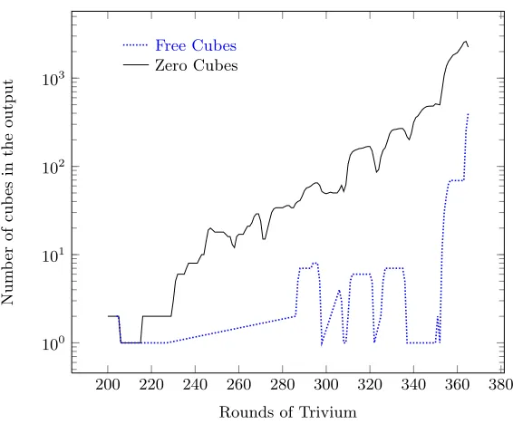
Fig. 1. Total number of zero and free cubes in the output of Trivium (rounds 200–365).
Fixing variables. Here we briefly discuss how fixing variables affects the residual polynomialr(V, K). Letµ be a monomial inr with|µ| ≥2. Moreover, we have some variablevi ∈µ. By setting vi= 0 the monomialµ will vanish. In addition, if µ was the only monomial with xC|µ in r this allows a new cubeC. On the other hand, settingvi = 1 leads to a new (restricted) monomialµ0 :=µ\{vi}. Assume that µ0 is already part of the initial residual polynomial r(V, K). In this case, the newly generated µ\{vi}will simply cancel outµ0 and hence may foster the existence of another cube. So both may be useful to generate cubes for a given functionf.
We want to stress that flexible cubes are a strictly weaker notion than free cubes: Fixing one additional variable in a free cube cannot destroy the cube-property. Any free cube is also a fixed cube for any assignmentα overV\C. Similarly, we can start with a flexible cube and fix up to|F|
variables until it becomes as fixed cube (or even a zero cube, if all variables become zero in α). This can be seen in figure1 as the number of fixed cubes exceeds the number of free cubes, except for rare cases where both number are equal.
From a cryptanalytic point of view, fixed/zero cubes are more desirable than free cubes as they are more frequent than the latter. Consequently, we have a higher probability of finding them. However, if we want to combine other attacks with cube attacks, free cubes or maybe flexible cubes are more interesting as we only take away variables from the cube-set C (or S, respectively). All other variables are still available for some other attack, cf. section2.6in the case of dynamic cubes.
2.5 State cubes
consequently taking advantage of its internal structure. We try to capture this with the following definition.
In this section let V be the space of the possible IV’s, K the key space andS the space of the states of a cipher. Denote u :V × K × S → S,(I, K, S) 7→ S0 the update funtion of the cipher. A cube inu or in a part of is called astate cube. They nicely relate to the Higher Order Differentials from Lai [Lai94].
The main goal of state cubes is to simplify the internal state of a cipher from an attacker’s point of view. In order to do so we need an algebraic modelling technique for the cipher that allow us to handle many instances of the cipher and than add some state bits. With this in mind we can simplify the state of the cipher symbolically. We will discuss this in more length in Section 4. A concrete example of state cubes is given there as well, cf. example 9.
2.6 Dynamic Cubes
Dynamic cubes were first described in [DAS11] where they were used to break full Grain-128. Dynamic cubes can be seen as a special case of free cubes. Let S ⊂ V be the set of all fixed variables in the original cube attack. We take a subsetD⊂S, called the set of dynamic variables. They are used to define a functiond(V, K) in the public variables and some key variables. Each such functiondis chosen in a way that some state bits cancel out. Alternatively, we can use the function
d to get some information of the cipher that can be used by cube testers. Finding the function
d requires a careful analysis of the internal structure of the cipher under attack. The following example is taken from [DAS11]. It illustrates the overall idea of dynamic cubes.
Example 4. We consider a polynomial P which is decomposed into P = P1P2+P3 where P1, P2
and P3 are polynomials overk1, . . . , k5 and v1, . . . , v5 with
P1:=v2v3k1k2k3+v3v4k1k3+v2k1+v5k1+v1+v2+k2+k3+k4+k5+ 1
P3:=v1v4k3k4+v2k2k3+v3k1k4+v4k2k4+v5k3k5k1k2k4+v1+k2+k4
and P2 is an arbitrary dense polynomial in the variables.
If we can force polynomial P1 to zero than P = P3. From the above definition we see that P1
is a rather simple polynomial. First we set v4 = 0 and make use of the linearity of v1 in P1 by setting v1 =v2v3k1k2k3+v2k1+v5k1+v2+k2+k3+k4+k5+ 1. This enforces P1 = 0. During
cube summation the value ofv1 will change. This is the difference between dynamic cubes and the definition of cubes as in Section 2.
Now we guess all values necessary to calculate v1. In particular, these are k1, k1k2k3 and k2+ k3+k4+k5+ 1 (!). Plugging in the forv1 and v4 we get:
P =v2v3k1k2k3+v2k2k3+v3k1k4+v5k3k5+k1k2k4+v2k1+v2+k3+k5+ 1.
2.7 Mixed cubes
Until now, we have worked within the framework of cubes. Here, we will provide an alternative, but nevertheless useful definition from a cryptanalytic point of view. Let O ⊂ V the oracle variables withO∩S =∅ and a functionf of the form
f(V, K) =xCp(K, O) +r(F, K).
If∀µ∈r :xC 6 |µ we callC a mixed cubes.
At first glance, this definition is not very useful as it mixes IV variables into the key equations of the superpoly. However, at second glance this changes as we can now reduce the dimension of the cube C: As long asxC -µ holds for all µ∈r, we can readily absorb variables from the set C into the set O and therefore reduce the cube dimension. In addition, we now have a much better source of (nonlinear) equations in the key variables: By setting the variables from O to different values, we obtain different (not linearly dependent) versions of the superpoly p(K, O). Basically, we can “switch on” different monomials in p(K, O) by setting the corresponding oracle variables to 1. Furthermore this new definition is less restrictive; consequently, we can expect more possible cubes and also cubes for a larger number of rounds than for the original definition of a cube.
To reflect this, we also need to change the definition of the key-degree of a mixed cube. It now becomes the maximal number of key-variables in any monomial in the superpolyp(K, O). Formally:
key-degree(f) := max
α:O→B{deg(p(K, O)|α)}
Example 5. ConsiderK :={a, b, c}, V :={α, β, γ}be the sets of key and IV variables, respectively. In addition, we consider the oracle variables {α, β} and the functionf :K∪V →Bas
f(K, V) := 1 +a+c+ab+αa+ +γa+γb+αγ+αγa+βγb
This leads to the following mixed cubes:
cube superpoly
∅ ab+a+c+ 1 +αa γ a+b+α+αa+βb
We see that the only “real” cube isγ. In addition, the superpoly corresponds to different equations, depending on the choice for the IV variables α, β. In particular we have
(β, α) superpoly (0,0) a+b+c
(0,1) b+c+ 1 (1,0) a+c
(1,1) c+ 1
So usingp(K,(1,1)) we can compute the value of the key variablec. Furthermore, usingp(K,(0,1)) and p(K,(1,0)) yields the values of of the key variablea, b.
2.8 Polycubes
Until now, cubes were only defined forcube monomials. In this section, we consider a generalization. Let C = {C1, . . . , Ck} be a set of k cubes with the corresponding superpolys p1(K), . . . , pk(K). Consider their sum
s(C) :=X i=1
kpi(K).
We calls(C) apolycube. In particular, for deg(s) = 1, we have a linear polycube.
Example 6. Following the notation of the other examples so far, we investigate the function
f(K, V) :=abα+abβ+aβ+aβγ+bβγ+bcα+bcβγ+βγ
Among others, this leads to the following cubes:
cube superpoly
α ab+bc
β ab+a
βγ bc+a+b+ 1
Considering the polycube defined byC={α, β, βγ}. This leads to the superpolys(C) =b+ 1. As its degree is 1 rather then 2 {βγ, β, α} it is more useful for cryptanalytic attacks than the individual cubes from C.
While polycubes are much more general than the other cubes treated so far, they are also much harder to find. For example, the algorithm from Section 3 can easily detect fixed cubes and even flexible cubes. However, it cannot find polycubes. Hence we have to state it as an open problem to give an efficient method to extract meaningful polycubes from a given cryptographic primitive, in particular when it is given in partial ANF (see below). Note that polycubes are a generalization of thecancellation attack from [Vie08].
2.9 Factor cubes
As before, we ease the restriction that the cube must be a single monomial. Instead of having a monomial, we use apolynomial σ(C). The defining equation of a cube now becomes
f(K, V) =σ(C)p(K) +r(V, K).
In a sense, the term σ(C)p(K) “factors out” f(K, V) +r(V, K), hence the name of this cube. In addition, we requireP
v∈ICσ(v) = 1 and P
v∈ICr(v, V\C, K) = 0. Using the same argument as for
theorem1, the latter condition becomes@µ∈r :xC|µfor a free factor cube and xC 6∈r for a fixed factor cube.
Example 7. As before, we haveK :={a, b, c}andV :={α, β, γ}. Moreover, we consider the function
f(K, V) := (α+β+αβ)(a+b+ 1) + (α+β+γ)(a+b+c)
Using the definition from above we obtain the cube polynomial σ({α, β}) = α +β +αβ, the superpolyp(K) =a+b+ 1 and the remainder r(K, V) = (α+β+γ)(a+b+c).
3 Trivium
To demonstrate our framework we use the stream cipher Trivium. It is a well-known hardware oriented synchronous stream cipher presented in [CP08]. Trivium generates up to 264 keystream bits from an 80 bit IV and an 80 bit key. The cipher consists of an initialisation or “clocking” phase ofRrounds and a keystream generation phase. There are several ways to describe Trivium— below we use the most compact one with three quadratic, recursive equations for the state bits and one linear equation to generate the output. The two only operations in Trivium are addition and multiplication over GF(2) as this can be implemented extremely efficient in hardware.
Consider three shift registers A:= (ai, . . . , ai−92), B := (bi, . . . , bi−83) and C:= (ci, . . . , ci−110).
They are called the state of Trivium. The state is initialized with A = (k0, . . . , k79,0, . . . ,0), B =
(v0, . . . , v79,0, . . . ,0) andC = (0, . . . ,0,1,1,1). Here (k0, . . . , k79)∈Bis the key and (v0, . . . , v79)∈ B is the initialization vector (IV) of Trivium. Recovering the first vector is the prime aim of attackers. Note that the second vector is actually known to the attacker. In cube attacks, we even make the assumption that an attacker can fully control the IV used within the cipher and obtain a stream of output bits for a fixed key and any choice of initialization vector (IV).
The state is updated using to the following recursive definition.
bi:=ai−65+ai−92+ai−90ai−91+bi−77 ci:=bi−68+bi−83+bi−81bi−82+ci−86 ai:=ci−65+ci−110+ci−108ci−109+ai−68
After a clocking phase of R rounds, we additionally produce one bit of output using the function
zi:=ci−65+ci−110+ai−65+ai−92+bi−68+bi−83.
Note that the three state update functions correspond to 3 linear feedback shift registers with 5 tap positions each. Each polynomial is irreducible over GF(2) and hence provides an LFSR of maximal period. In each LFSR, the second-last term has been replace by a quadratic monomial. This is the only non-linear component in Trivum. Our results are based on round-reduced versions of Trivium with special choices ofR. Full Trivium usesR = 1152 initialization rounds. Until now, no successful attack is known against full round Trivium.
There exist further variants of Trivium using two instead of three shift registers [CP08]. They are called Bivium-A and Bivium-B.
3.1 Brief overview of attacks on Trivium and round-reduced Trivium
The attacks from [DS09a,FV13] are both cube attacks. They recover the full key of a 799 round-reduced variant of Trivium in 262computations. Nevertheless, more attacks on Trivium are known
so far. In [KMNP11,ADMS09,Sta10] their are some distinguishers attacks based on cube testers that cover up to 961 rounds but only work in a reduced key space of 226 keys. Time complexity is 225 computations.
Pure algebraic attacks are given in [SFP08,T+13,SR12,Rad06]. They break the both reduced variants Bivium-A and Bivium-B. They fail for Trivium, even in its round-reduced version. Main reason is that they all begin their attack after the initialization phase so they are limited to one instance of Trivium.
Other attacks are not as succesful. For instance [KHK06] contains a linear attack on Trivium breaking a 288 round-reduced variant with a likelihood of 2−72.
4 Similar variables and state cubes
The cube attack as defined in [DS09a] views the corresponding cipher as a black box. So there is no chance to take the initialisation phase of a given cipher into account. Thus cubes are limited to the output of the cipher; consequently, if we do find cubes for the output of the full cipher the attack fails.
By Kerckhoff’s principle, we actually know which cipher we attacking, so we can overcome this disadvantage by building a suitable algebraic model. Here we do this exemplary on the stream cipher Trivium. However, the presented modelling technique is by no means limited to this cipher.
Algebraic attacks in [SFP08, T+13, SR12] are based on the same algebraic representation of Trivium, namely the one given in [Rad06]. So all state bits of one Trivium instance are set to symbolic variables after the initilization phase. In the first model they intoduce three new variables for ai, bi and ci every time the output is generated; we denote the number of output bits by no. Based on the above defintions, they obtain a sparse quadratic system of equations with 288 + 3∗no variables and 4∗no equations . In the second model the authors of [Rad06] do not introduce any intermediate variables. Therefore the equations are of ascending degree in the 288 state bits and the system of equations becomes dense. Consequently, it is also much harder to solve. All in all these strategies have limited success as they broke Bivium-A and Bivium-B but did not manage to break Trivium or even round-reduced versions of Trivium.
Our goal is to use cubes which occur in the state bits of Trivium. Therefore we need an alge-braic representation that can both handle more than one Trivium instance and is also able to use information from the internal state.
To this aim, we only use symbolic values of the key variables. Then we update Trivium a number
R of rounds only generating intermediate variables when we need them to bound the degree of the equations by two. This allows us to generate many Trivium instances with the same key but with different IV vectors.
4.1 Algebraic representation using similar variables
LetI ⊂V be a subset of the IV variables. We consider the firstnooutput bits of Trivium instances that are all defined by the same key and all vectors fromIS for some fixed set S, cf. the definition of IS in section 2.1.
In our approach we set up all Trivium instances with symbolic variables k0, . . . , k79 for the key
and set the IV variables corresponding to vectors in B|S|. Denote the current Trivium instance by
t∈N. We initialize these instances for a given number of roundsRand introduce three new variables every round for the entries at,i, bt,i and ct,i in the three Registers At, Bt and Ct. This produces a quadratic system with a large amount of variables and monomials. Therefore we introduce some methods to reduce the number of variables. This reduction of the number of variables and monomials is important because solving techniques such as Gr¨obner-bases algorithms depends heavily on the number of variables. First of all we consider one Trivium instance in the following lemma.
Lemma 1. Let R >238 and no 666. With the algebraic modelling technique described above we use exactly 3R−522intermediate variables to describe one Trivium instance.
Proof. We want to count the intermediate variables generated while modelling one Trivium instance. To do so we consider the update function
bi=ai−65+ai−92+ai−90ai−91+bi−77 ci=bi−68+bi−83+bi−81bi−82+ci−86 ai=ci−65+ci−110+ci−108ci−109+ai−68
of Trivium. Whenever we would get an equation of total degree greater than two we set the quadratic equation to a new intermediate variable and continue the calculation with it. Our proof deals with each registerA, B, C one after the other.
At the begining register A is the only one containing symbolic values. In the 13th round the first quadratic expression b12=a78·a79+· · ·=k79·k78+· · · is produced. Inspecting the update
equations of Trivium, we see that it takes 82 rounds until it will be multiplied in round 94 with a linear element inc95 and the first intermediate variable will be introduced. After round 94 we use
one new variable in the register C every round.
We count the intermediate variables in the other registers in an analogous fashion. First we consider registerA. The above mentioned quadratic expressionb12 will also be stored in registerC
in round 13 + 69 = 82 because of c80 =b12+· · ·. In round 191 this expression will be multiplied
with an linear expression in a189 = c81·c80+· · · and we have to introduce a new intermediate variable in the register A. Thus after round 190 there will be a new variable in registerAandC in each round.
Now we investigate the registerB. As mentioned above our quadratic expression b12will stored in registerC in round 82. After 66 more rounds it is stored ina145=c80+· · ·. From there it takes further 91 rounds until a new variable is required inb236 =a146·a145+· · ·. So starting in round 239
we will need a new intermediate variable in every register without further reduction techniques. So all in all, we have the following numbers of intermediate variables ν:
ν = (R−94) + (R−190) + (R−238) = 3R−522.
output function of Trivium
zi =ci−65+ci−110+ai−65+ai−92+bi−68+bi−83
is linear and uses at most 66 rounds old state bits. Thus we do not have to clock the registers and so do not introduce new intermediate varibales if we wantno 666 output equations. ut
Corollary 1. For 0 6no 6 66 output bits, we need to compute only R+no −66 updates of the state in Trivium.
For the remainder of this section we assumeR >238. Now we take a more general point of view and introduce similar variables for generalized systems of equations. Nevertheless we will later on use this observation for a system of many instances of Trivium.
Definition 1. Let R = F2[k0, . . . , k79, y0, y1, . . .] =: F2[K, Y] be the Boolean Polynomial Ring in
the key VariablesK and all intermediate variables Y.
We call two intermediate variables yi and yj similar iff yi +yj = p(K, Y\{yi, yj}) where
p(K, Y\{yi, yj}) is a polynomial of degree deg (p)61.
Taking similar variables into account we can save many intermediate variables. Whenever we want to introduce a new intermediate variable we first test if there exists a similar one. If yes, do not introduce a new one but useyj +p(K, Y\{yj}) instead.
Furthermore if we have the set F of polynomial equations in R introducing the intermediate variables, the so-called set of system equations, we can generalize the definition above as follows:
Definition 2. Let R = F2[k0, . . . , k79, y0, y1, . . .] =: F2[K, Y] be the Boolean Polynomial Ring in
the key variables K and all intermediate variables Y. Denote with F the system equations. Denote by Yk⊂Y, Yk 6=∅ for 1≤k <|Y| the sets of already introduced intermediate variables up to stepk. We call the intermediate variableyi similar to the setF iff there exist a non-empty set
Yk such thatyi+Py∈Yky=p(K,(Y\Yk)\{yi}) where p(K,(Y\Yk)\{yi}) is a polynomial of degree
deg (p)61.
The following example illustrates how we work with similar variables.
Example 8. Consider the equations defining intermediate variables
y0=k78k79+k53 y1=k77k78+k79+k52
in the system of equationsF. Assume we want to introduce the new intermediate variable
y2=k79k78+k78k77+k5+k61.
We havey2 =y1+y0+k53+k79+k52+k5+k61. So we do not needy2 and we can go on computing
withy0andy1 instead. This does not only save us one variable but we also have replaced a quadratic equation by a (potentially more useful) linear one.
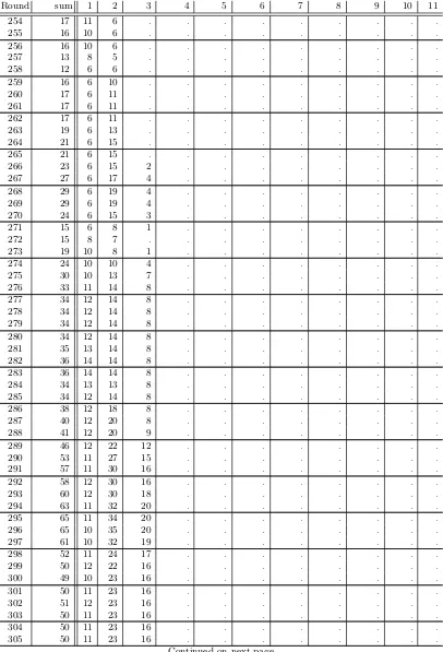
Table 1.R: Number of initial rounds, 3R−522: One instance without similar variables,ν: number of intermediate variables; the number of output bits is set to 66 and 32 Trivium instances are generated.
R 3R−522 ν
400 678 548 450 828 961 500 978 1489 550 1128 3510 600 1278 6557
The first column of Table1gives the number of initialization rounds for each Trivium instance. In the second one we have the number of variables used for one Trivium instance without similar variables and the number of intermediate variables which are used to describe the whole system isν. We see that have greatly decreased the number of variables. Usually we would need 1278∗32 = 40896 variables to model 32 instances 600-round-reduced version of Trivium. We also have produced 66∗32 = 2112 output equations. The model in [Rad06] can just handle one instance and needs 288 + 3∗2112 = 6624 variables to produce that amount of output equations. In our model we see a saturation of the number of variables and monomials. We discuss this point in more depth later in this article. Thus increasing the number of instances actually increases our advantage, too.
These systems are out of reach for nowadays Gr¨obner bases implementations like PolyBoRi [BD09]. The number of variables is simply too high.
We describe algorithm 1. It is used to generate the model outlined above, but is specialized to Trivium. Algorithm 1 returns a system of equations F that representT ∈N instances of Trivium withR rounds andno666 output. The key variablesk0, . . . , k79are shared among these instances.
However, the IV variables vt,0, . . . , vt,79 are initialized with different values for each individual
in-stance. In the function representation the three shift registers are initialized and output is produced according to the functionupdateStatefor thet instances of Trivium. After setting up the system
F we echelonize it by interpreting it as a matrix with monomials as columns and polynomials as rows. The echelonized form creates two sets, namely quadratic equations Q and linear equations
L. Using the linear terms from L, we can simplify Q. To this aim, we replace the leading terms LT(L) ofLinQby their corresponding equations. In doing so we useDegree Reverse Lexicographic ordering with a round ascending ordering and put key variables first. In this case, echelonizing and plugging in LT(L) in Qdirectly makes use of similar variables. This follows as the echelonization algorithm first puts intermediate variables of higher rounds before those of lower rounds. All linear relations are then used to produce even more similar variables. insertLinVars is plugging these linear equations into the rest of the equation system.
Before discussing the running time of the algorithm 1 we note that it can be applied to other ciphers as well. When other ciphers have a quadratic update function, we can directly apply algo-rithm1. Otherwise, we need to take care of the higher degree of the update function.
Algorithm 1 Generating the algebraic representation of Trivium F using similar variables. The function echelonize echelonize the matrix coresponding to F and insertLinVars plugs the linear variables into the systemF
1: functionupdateState(k, out): 2: if out =true then
3: F.insert(ci−65+ci−110+ai−65+ai−92+bi−68+bi−83)
4: return
5: end if
6: F.insert(at,k+A[0]);F.insert(bt,k+B[0]);F.insert(ct,k+C[0]) 7: A[0]←at,k;B[0]←bt,k;C[0]←ct,k
8: forj←0to91do
9: A[j+1] = A[j] 10: end for
11: A[0] =ci−65+ci−110+ci−108ci−109+ai−68 12: forj←0to82do
13: B[j+1] = B[j] 14: end for
15: B[0] =ai−65+ai−92+ai−90ai−91+bi−77 16: forj←0to109do
17: C[j+1] = C[j] 18: end for
19: C[0] =bi−68+bi−83+bi−81bi−82+ci−86 20: return
21:
22: functionrepresentation(R, no, t): 23: globalF← ∅
24: forn←1totdo
25: globalA←(k0, . . . , k79,0, . . . ,0);B←(vt,0, . . . , vt,79,0, . . . ,0);C←(0, . . . ,0,1,1,1) 26: fork←0toR−1do
27: updateState(k, out=false) 28: end for
29: fork←1tonodo
30: updateState(k, out=true) 31: end for
32: echelonize(F) 33: insertLinVars(F) 34: end for
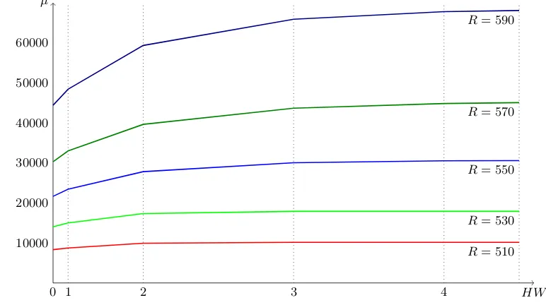
Fig. 2. Saturation of variables; Hamming Weigth against number of variables for R rounds of Trivium
HW ν
0 1 2 3 4
1000 2000 3000 4000 5000
R= 500
R= 520
R= 540
R= 560
R= 580
The matrix corresponding to F is anm×n−matrix where n is the number of monomials and
m is the number of equations in F. In the update function there will be at most 3 new equations per round. After 111 rounds these polynomials consists of 4 monomials each. So there are more monomials than equations since we haveR >238. As a consequence the running time of step 2 can be approximated byO(n3). Note thatngrows per instance we generate. As we will see below, the number of variables and monomials saturates.
The functioninsertLinVarshas a running time ofO(n2p·m). We have to insert allmequations of the system to at most the maximum number of monomials np inone equation in F.
We get an overall running time of O(T n3) since the echelonization is the most expensive step and we perform it at mostt times.
In practice, this number will be lower. For example, we can use an implemenation of Strassen’s algorithm So the running time is more likelyO(T n2.7) orO(T n2) as long as the systemF is sparse.
Saturation. We can see in figures2–3that similar variables greatly effect the number of variables. In our experiments we found a saturation of the number of variables and monomials that depends on the Hamming weight of the IV we are using and on the initialization roundsR.
When generating many instances we takeiIV bits and produce the 2i instances corresponding to all possible vectors from Bi. When generating an instance of high Hamming weight we spend less variables and monomials than for an instance of low Hamming Weight. When the number of rounds grows we need to generate more instances to see this effect. We have plotted this effect for 32 instances in figures 2–3, counting both the number of variables and the number of quadratic monomials.
Fig. 3. Saturation of monomials; Hamming Weigth against number of quadratic monomials forR
rounds in Trivium
HW µ
0 1 2 3 4
10000 20000 30000 40000 50000 60000
R= 510
R= 530
R= 550
R= 570
R= 590
Hamming weigth against the number of quadratic monomials µ in F. All in all, the saturation of monomials is much flatter then the saturation of variables. Note that variables that are not saturated are found in the linear terms.
This means that at some point we get more system defining equations from the output than new variables or monomials. So our system gets defined or even overdetermined when we have enough instances. Note that we did not take the output equations into account yet but only the defining system itself. The output introduces additional, unknown monomials but no new variables.
4.2 Taking advantage of the white box
With the modelling techniques described above we are able to obtain the symbolic values for any state bit in any round from any instance of Trivium. This allows us to (cube) sum certain state bits from different instances to form state cubes (see section 2.5).
First we note that similar variables generate cross references between all instances we produce. Second, we directly obtain linear equations in the key variables and use them to obtain more similar variables. Finally, if the number of rounds is low enough, we even get linear equations between the output and key variables. In this case, we can simplify the system even further.
Now we have access to a full symbolic state so we can add state bits from many instances. This is one assumption of the cube attack. The second one is the existence of cubes in the state. How to find cubes is stated in section 5. With these techniques we found many state cubes. Detailed results are given in section 6.
For reference: Until round 699 we have found about 31,000 state cubes within the first 12 IV variables. We have used the algorithm from Section 5.4 for this search. Note that state cubes do not lead to a linear system in the key bits. They establish more cross references between the key bits and the state bits from initialization rounds. So when we have assembled enough state cubes in the systemF we skip even further initialization rounds. When we have a full representation of the cipher using algorithm 1we can use it to generate additional equations from known state cubes.
Example 9. To see that state cubes actually exist, consider
state/round Cube superpoly
b302 v0 k65
a350 v11 k15
b546 v0v1v3v9 k55+k61 c586 v0v1v2v3v4v5v7v8v9v11 k9 a601 v0v2v3v4v5v6v7v8v9v11 k65
Also these examples are completely arbitrary taken from the list of possible state cubes, they can be used to illustrate the idea: Take b302. This leads to the equation
b0,302+b1,302+k65= 0
that is valid independent of the choice ofk65. By replacingb0,302andb1,302with their corresponding
representation inki, yj, we obtain a new equation that we can add to the overall systemF.
5 Cube finding
The main technique for finding cubes in a given cipher isblack box polynomial testing. This means we view the corresponding function as a black box and try to interfere a (partial) ANF and consequently cube equations. Most successful for this purpose are a random-walk algorithm [DS09a] and its successor [FV13]. The latter uses additional memory to speed up the computation. For the sake of simplicity, we only state the former for the case of linear cubes.
Random Walk Algorithm. We start with a random set C ⊂ V and compute the superpoly p(K) by multivariate polynomial interpolation. There are three possible outcomes: the degree ofp(K) is 1. In this case, we output the pair (C, p) as a new cube/superpoly. Alternatively, the degree may be zero or negative. In this case, the set C was too large and we drop one element from it. If we cannot compute a linear superpoly, its degree is higher than 1 and we need to add another variable to the set C. If we do not succeed after a certain number of trials, we restart with a fresh setC.
Unfortunately, the analysis of both algorithms is rather tricky, so we do not know how many / which type of cubes they will find. Consequently, we cannot make statements like “Trivium does not have cubes of dimensionkin roundr” but only “Our algorithm did not find anything (yet)”. In particular, there is quite some freedom in choosing the “correct” starting setC and also to include / drop certain variables which further complicates the situation. This is obviously an obstacle to develop a full theory of cubes and their existence in cryptographic algorithms.
5.1 Polynomial degree testing
As linearity testing and its generalization to higher degree polynomials are an important building block, we state the degree testing algorithm from [BLR93] both in its generalized form and in its (easier) linearized form. We start with the latter. Let f(x) : GF(2)n → GF(2) be a Boolean function. We want to establish with high probability if f is linear,i.e. (1) holds.
∀x, y∈GF(2)n:f(x+y) =f(x) +f(y) +f(0) (1)
If the function f is available in full ANF, this is easy. However, if f is only available in black-box-access, the problem becomes difficult. A possible way out is the one-sided BLR linearity test [BLR93]. Here, we evaluate (1) for several, randomly chosen pairs (x, y)∈RGF(2)n×GF(2)n. If (1) is violated by at least one pair, we conclude thatf isnot linear. To confirm thatf is indeed linear with probability 2−s for some certainty levels∈N, we need a total ofd(4 + 1/4)serepetitions.
Algorithm 2 Compute the degree of a given function f. The degree must be within the set of target degrees D. Otherwise, return⊥
1: functionaddSet(X): 2: if |X|= 0then
3: return 0 4: end if
5: a= 0
6: for allx∈X do
7: a←a+x
8: end for
9: return a
10:
11: functioncomputeDegree(f, D, s) 12: d←max(D);r←0
13: whiler <
d2d+ 1 2d+1
s do
14: x1, . . . , xd+1∈R GF(2)n
15: A= (. . .){Empty sequence}
16: for all σ⊂ {1, . . . , d+ 1} do
17: Aσ←f( addSet({xi:i∈σ})) 18: end for
19: D0← ∅
20: {Iterate over all potential degrees}
21: for allδ∈D do
22: {Iterate over all subsets of lengthδ}
23: for alls∈ {b⊂ {1, . . . , d+ 1}:|b|=δ}do
24: if addSet({Aσ:σ∈s})6= 0then
25: D0←D0∪ {δ} {We found a witness against degreeδ}
26: end if
27: end for
28: end for
29: D←D\D0
30: if |D|= 0then
31: return ⊥
32: end if
33: d←max(D);r←r+ 1 34: end while
In a more general framework, i.e. assuming that we want to confirm that f has degree dwith probability 2−s, we need a total of
d2d+ 1 2d+1
s
repetitions of the above test. The corresponding lemma and algorithm are given in [JPRZ09]. Instead of stating it here, we further generalize it from degreetesting to degree detection, that is, given a function f we determine its degree within a given range. See algorithm 2 for the pseudo-code. In particular, linear and quadratic functions (so d = 1,2) are of high interest to us as they correspond to linear and quadratic cubes. Although such an algorithm seems to follow directly from the one given in [JPRZ09], there are some subtilities that allow a considerable speed-up in practice. In particular, we can save on (expensive) evaluations of the underlying function f by re-arranging them into different subsets (lines 23–27). This is possible as all values are chosen pairwise independent.
All in all, the algorithm samples d2d+21d+1
s(d+ 1) random vectors from the vector space
GF(2)n and needs ( d2d+2d1+1
s)2d+1 = O(ds22d+1) evaluations of the underlying function f. Consequently, it is not suitable to extract the degree of a large number of quadratic or even cubic cubes. As we will see in Section 5.5, this function is the real bottleneck when searching for a large number of cubes. So one of our goals is to develop more efficient filters to limit the use of the above algorithm to the absolute minimum. On the up side, the linearity tester can readily be parallellized as we can distribute different cubes to different machines with only minimal communication overhead.
5.2 Basic algorithm
In any case, when looking for cubes we are searching a needle in a hey-stack. Even worse, when using one of the random walk algorithms, we push the search in a certain direction. Therefore, “real” cubes might have different properties than the ones we find by these algorithms. To overcome this problem, we will discuss several algorithms that capture cubes more accurately. In particular, we have a tighter control over the probability space they operate on, so we can make better funded claims, e.g. about the distribution of cubes within Trivium.
The first algorithm is rather trivial, but nevertheless useful—both for Trivium up to round 446 (cf. Section 5.5) and also as a building block for further algorithms. In a nutshell, we use the full ANF of the corresponding function and then apply the corresponding cube criterion from Section 2. Although we could use any of the above criteria to determine the existence of a cube, we have specialized the algorithm to the case of linear zero (fixed) cubes as they have the highest relevance for direct cryptographic attacks. In addition, this eases explanation of the general idea.
The subfunction split is used to separate key variables from IV variables for a given mono-mialµ. Based on this, we add up all superpolys in lines 5–9. By definition, we only allow superpolys of degree 1 or lower. These are extracted in line 11.
Correctness. The correctness of the algorithm follows from the definition of fixed linear cubes: Start-ing with the ANF of f, we regroup all monomials by their IV variables. Adding all key-variables for a givenxC yields the corresponding superpoly (line 7). Excluding the one-monomial∅(line 10), we just need to test which potential superpoly actually has the correct degree (line 11).
Algorithm 3 Directly extracting cubes from a functionf, given in Algebraic Normal Form
1: functionsplit(µ)return(µ∩V,µ∩K) 2:
3: functionextractCubes(f)
4: superPolys←(0, . . . , 0); potentialCubes← ∅
5: for allµ∈fdo
6: ν, κ←split(µ)
7: superPolysν ←superPolysν+κ
8: potentialCubes.insert(ν) 9: end for
10: potentialCubes←potentialCubes\{∅}
11: allCubes← {ν∈potentialCubes : superPolysν.degree() = 1}
12: returnallCubes
Example 10. Let K := {a, b, c}, V := {α, β, γ} be the sets of key and IV variables, respectively. Moreover, consider the following function f :K∪V →Bin algebraic normal form (ANF):
f(K, V) :=abα+aαβ+aβ+aβγ+bβγ+cαβγ+bcα+abcαβ+abcαγ+bc+a+b+βγ+ 1
Using algorithm 3, we have the following superpolys, indexed by IV sets:
IV setν superPolysν linear
∅ bc+a+b+ 1
-α ab+bc
-β a ?
αβ a+abc
-αγ abc
-βγ a+b+ 1 ?
αβγ c ?
So consequently, our algorithm returns the set {β, βγ, αβγ}. Although not a linear superpoly,
bc+a+ 1 is interesting, too. We note that the corresponding cube ν = ∅; by definition, this corresponds to the monomial 1. It will occur in the cube summation of every other cube. In our case, this is the ANF of the restricted functionf(K,(0,0,0)) =bc+a+ 1. In practice, this special form of the function f will exist for any given cipher, but has a far too high algebraic degree to be of practical use. Therefore, we rely on the fact that f(K,(0,0,0)) is summed an even number of times and hence cancels out in the cube sum.
Running time. Its running time is bounded from above by the number of monomials inf and the length of the longest monomialµinf. Denote these with |f|and|µ|. Then both the running time and the memory consumption are inO(|f||µ|).
5.3 Pushing the limit
Up to now, we were dealing with the full ANF of the target functionf. For cryptographic algorithms, this becomes prohibitively expensive as the degree off (and also the number of monomials) usually increases exponentially, cf. section 6.1and in particular figure4 for the case of Trivium. Note that this is primarily a concern of the available memory, not so much of the available running time.
A simple but effective trick to reduce memory consumption is to evaluatef in some IV variables by simply setting them to zero. We denoted the result byf. So instead of using algorithm3with the full functionf, we usef as its input. In the remainder of this section we investigate the implications of this approach.
First, this idea has some similarities to the random walk algorithm. Here, we start at some random point and evaluate f “around” it. But it also has some advantages over the latter. In particular, our restriction is independent from the search algorithm so we can better control it. Consequently, we can easily estimate the number of cubes thatshould live at the evaluation off in a given round, cf. lemma 2. Running the algorithm several times and combining the observations of several such restrictions increases the accuracy of the prediction. Note that this algorithm is particularly well suited for fixed cubes. Considering both the search space and the overall space of IV variables leads to the following lemma:
Lemma 2. Let R be the number of cubes of dimension r ≥1 in a function f(K, V). Let f be its restriction such that we have f(K, V) for V ⊂V. Then we expect on average a total of
R·(|V|/|V|)r
cubes of dimension r in f.
Proof. For the proof consider some cube C of dimensionr and a randomly drawn set V ⊂V. For each variable in C we have a probability of |V|/|V|that it is also contained in the set V. As all these r events are independent, the lemma follows for one cube and consequently for all R cubes inV.
However, to succeed in practice, we cannot compute the function f and then restrict it. This is impossible to the memory constraints. But if f is recursively defined, we can do it the other way around: First assign values to all corresponding variables and then develop f following its definition. This will lead to the same function f. Note that such a recursive definition exists for Trivium in particular and also for all relevant cryptographic functions. For example for the AES, this was made explicit in [MR02, CMR05]. Similar work has been done for Present [Lea10] and other cryptographic primitives such as SHA-3; for this, we can use the so-called “Keccak-Tools”, to generate the corresponding equations explicitly, including round reduced SHA-3.
Example 11. Using the same functionf as in example10, we chooseV ={β, γ}. Consequently, the restricted functionf becomes:
f(K, V) :=aβ+aβγ+bβγ+bc+a+b+ 1 +βγ
Using algorithm 3, we have the following superpolys, indexed by IV sets:
IV setν superPolysν linear
∅ bc+a+b+ 1
-β a ?
As expected, the algorithm cannot identify all cubes anymore and the resulting set becomes now
{β, βγ}. By also considering V1 ={α, β} and V2 ={α, γ}, algorithm 3 we would actually find all
cubes up to dimension 2.
Correctness. Using the ANF of the functionf for the sake of the argument, we see that restricting
f to some subset V of IV variables will destroy all cubes that contain at least one variable outside of this set. On the other hand, all cubes that are fully inside the set V will still be found. As this change does not affect the key variables, all superpolys are untouched. Hence, they will be correctly identified as linear, quadratic, . . . Using lemma 2 we see that we will only find a fraction of all possible cubes, namely (|V|/|V|)r for a given cube dimensionr.
Running time. Giving an exact formula for the running time of the algorithm presented in this section is difficult. However, we can use the same argument as for lemma 2 to see that for any given monomial ν∈f we only have a probability of (|V|/|V|)|ν| that this monomial is also present in f. As in Section 5.2, the running time depends on the length of the largest monomial|µ| and also the number of monomials in the ANF of the functionf, denoted by |f|. More specifically, we have a running time of O(|µ||f|). As both factors are reduced by at least |V|/|V|, we can expect a reduction in time and memory in the order ofO((|V|/|V|)2). Without having more information
about the actual monomials in f, it is not possible to obtain a more accurate bound. To make things worse, the polynomials we are dealing with are also structured. In particular this means that specific subsets of variables can occur much more frequent in the monomials of f than others. So for some choices of V, our reduction might be much less than expected.
In the case of Trivium, we have replaced the initial functionf in 160 variables and (potentially) up to 2160monomials by a functionf with 80+16=96 key and IV variables. Note that this algorithm is still fully deterministic but cannot find all possible cubes anymore. As we will see in section5.5
this is only feasible for small cube dimensions. However, we introduce a cube finding algorithm that can cover a higher number of rounds in the next section.
5.4 Going probable
Up to now, we have deterministic algorithms that allows us to find cubes for a given function f
or f, respectively. Still, we can increase the number of rounds we cover by further reducing the number of monomials. As we have dealt with the IV variables in the previous section, we will now concentrate on the key variables. We denote the result by f(K, V) or simply f. In the case of Trivium, we have a total of 80 key variables, so we can expect a noticeable gain by reducing them. Unfortunately, the situation is more complicated than in the previous section. By removing key variables, we are actually tempering with the superpoly and therefore destroying relevant information such as its degree. Still, we can construct a tester that will output (with some small probabilityρ) that a given set of IV variabesν ∈V inf isnota cube by looking at the corresponding structure inf. By repeatedly applying this tester on different double-restricted functionsf1, f2, . . .
we can turn this into a tester that detects non-cubes with overwhelming probability.
Algorithm 4For a given functionf, compute a list of plausible cubes. Parameters are the sub-set of cubes V, the number of key variables in the test setsκ, and the number of repetitions r.
1: functiondoubleF(V , K):returnf(V , K) 2:
3: functionplausibleCubes(f,V,κ,r) 4: noCubes← ∅; maybeCubes← ∅
5: fori←1tordo
6: K∈R{s⊂K:|s|=κ} {Get a random subset of sizeκ}f←doubleF(V , K)
7: superPolys←(0, . . . , 0); potentialCubes← ∅
8: for allµ∈f do
9: ν, κ←split(µ)
10: superPolysν←superPolysν+κ
11: potentialCubes.insert(ν) 12: end for
13: noCubes←noCubes∪ {ν∈potentialCubes : superPolysν.degree()>1}
14: maybeCubes←(maybeCubes∪potentialCubes)\noCubes 15: end for
16: returnmaybeCubes
Letp(K)xC be some superpoly and cube in function f. Assuming xC ⊂V, the superpolyp(K) becomes p(K). Consequently, some monomials in p(K, V) may be missing in its double-restricted version. On the other hand,p(K) being of degree 2 or higher is awitness forp(K) being of degree 2 or higher. To see the limits of our algorithm, we considerp(K) be monic and having degree|K|+ 1. No choice of K would reveal such a p(K) in p(K). Still—it is the same kind of error as above, so if p(K) has degree 2 or higher, p(K) is not a superpoly and xC is certainly not a cube. Still, our algorithm will not detect it. On the other hand, the likelyhood that p(K) has such a structure is very low, so we can detect this case via the degree testing algorithm from section5.1.
Example 12. Using the same functionf as in example10and the two setsK1 :={a, b}, V :={α, β}
of key and IV variables, respectively, we obtain the following function f in ANF:
f(K1, V) =abα+aαβ+aβ+b+a+ 1
Using algorithm 4, we have the following superpolys, indexed by IV sets:
IV setν superPolysν linear
∅ a+b+ 1 ?
α ab
-β a ?
αβ a ?
We see that all but one set is identified as possible cubes, namelyR1 ={∅, β, αβ}. However, consider
the following set of key variables K2 :={b, c} we obtain the new function
f(K2, V) =bβγ+bcα+bcβ+bc+a+b+βγ+ 1
IV set ν superPolysν linear
∅ bc+ 1
-α bc
-β 0 ?
αβ 0 ?
This leads to the new result R2 ={β, αβ} and consequentlyR =R1∩R2 ={β, αβ}. In order to
obtain the correct output {β}, we would need to consider the monomial abc, too. Assuming that we cannot develop an ANF with three key variables, we will need to leave this to the degree testing algorithm 2. Hence, we can use algorithm 4as a filter to identify potentially interesting regions of the overall function f.
Correctness. To see the correctness of algorithm 4, we inspect the ANF of a given functionf. For each choice of IV variables V and key variables K, we implicitly set all other variables to zero. Consider the sets ˜K := K\K, ˜V := V\V and the partial assignment τ : ˜K ∪V˜ → 0 that sets these variables to zero. So we deal with the functionf := f(τ, K, V). All monomials that contain at least one variable from τ become zero. Consequently, our algorithm will not see them. On the other hand, superpolys that can be expressed solely with variables from the setK over cubes from the set V will still be found. Hence, our algorithm is a one-sided tester. The probability can be computed using the same ideas as in lemma2.
Running-Time. As in the previous section, it is difficult to give a closed formula for the running time of the algorithm. However, we can give two sensible bounds on the probability that our algorithm actually outputs a witness. We first bound this probability from below in (2) and then from above (3).
First assume that onlyone coefficient of the superpoly is quadratic, all others are linear. In this case, we need to cover this monomial with our r sets and obtain
| ∪r
i=1{ab:a, b∈Ki}| |K|
2
(2)
as lower bound. In theory, we could also assume that p(K) has no quadratic but only one cubic monomial. In practice, this is very unlikely and was not confirmed in our simulations. Still, from a purely theoretical point of view, a probability of zero may be justified here: In this case, p(K) has degree |Ki|+ 1 but no monomials of degree 2, . . . ,|Ki|.
On the other hand, we will very likely have a more friendly shape of p(K). Here we assume that for all monomials inKi that it being present inp(K) with probability 50%. This corresponds to the case wheref is well developed in these monomials. This is particularly true for small cube dimensions. Hence we obtain as an upper bound
1−
1− |K|+ 1
2|K|
r
(3)
that a non-linear superpoly is caught by our test. In either case, our practical probability ρ is bounded by both equations and we obtain
Note that ρ is a function both of the cube dimension |C| as well as for the current round. So ρ
will increase from round to round until we have ρ = (3). On the other hand, increasing the cube dimension|C|will lead toρ= (2). Unfortunately, the correct value depends on the overall structure off. Hence, the only realistic way to compute the probabilityρ in practice is empirically. All in all, repeating the above test around 80 times gave us a success probability of about ranging from 99% to 30% thatC was actually a cube. As expected, the probability was higher for lower rounds than for higher rounds. This was verified with the standard cube test from Section5.1. More importantly, this cube test has an intrinsic running time of 2|C|, so precomputing plausible candidatesC1, . . . is
a good way to find all cubes for a given set of IV variables V and cutting down the running time of the combined algorithm.
5.5 Practical implementation
All algorithms from this section were implemented as a hybrid programme in both the computer algebra system Sage [S+13] and the programming language C++; the latter contains the more time-critical parts such as the cube linearity test. In total, the programm consists of 1500 lines of Sage code and the C++ part of around 900 lines of C++ code; both counts include comments.
Using the algorithm4with parameters|V|= 15,|K|= 6 and 80 iterations per cube, we searched for cubes up to round 570 in Trivium. For example, in round 550 this took around one hour (AMD Opteron [email protected]).
Verifying all plausible cubes took up to one additional core-month per round. Consequently, the work was distributed to a cluster with 256 cores and 1TB of RAM. Interestingly, with the above parameters, we could go on forever as the total number of variables per iteration is only 21. Alas, from round 570 on, there are no cubes left with 15 or less IV variables. On the other hand, reducing the number of key bits from 6 to 5 (or even lower) gave us too many false positives that the algorithm became unusable in practice. Unfortunately, the implementation consumed a lot of disk space (up to 1.2TB), so we could not increase the number of variables or iterations further.
In contrast, using the exact algorithm 3, we were able to fully cover the first 446 rounds of Trivium. To this aim, we needed to process a Boolean function with around 50 million monomials. To put this into perspective: A single state bit in round 399 needs around 2.7 GB of disk space and consists of about 82 million monomials with a total of 675 million appearances of the 160 variables from K∪V. Unfortunately, Sage and in particular its polynomial package PolyBoRi [BD09] are not able to deal with these high numbers of monomials / variables, so PolyBoRi repeatedly and predictably crashed. To conclude: memory was the real bottle neck for this algorithm, not time. The most promising way seems a full rewrite of the algorithm in C++. This also includes the development of a more compact representation of the monomials.
200 250 300 350 400 450 100
101 102 103 104 105 106 107 108
Rounds of Trivium
Num
b
er
of
cub
es
in
the
output
Cubes
Monomials
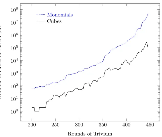
Fig. 4. Both the number of cubes and also the total number of monomials in the output function
f(V, K) of Trivium, plotted against the number of rounds.
6 Practical Results on Cubes
We now use the algorithms from the previous section to get some insights on the distribution of cubes for Trivium. This also serves as a test to see if both definitions and algorithms are actually useful in practice. All results were obtained on the computing cluster described in Section 5.5.
6.1 Cubes in the output
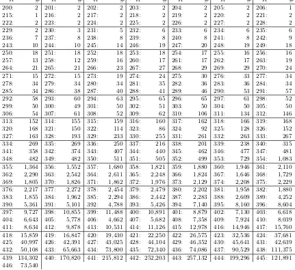
In figure 4 (cf. also table2) we see the total number of cubes in the output function
zi =ci−65+ci−110+ai−65+ai−92+bi−68+bi−83
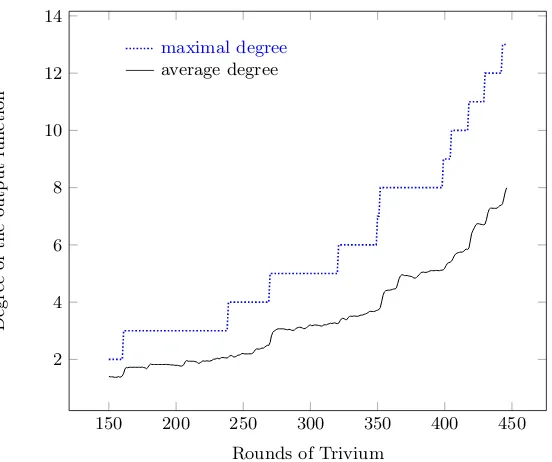
of Trivium for 200 ≤i < 447. Note that values below 200 are of only limited interest and hence not plotted here. This figure was computed with algorithm 3. Therefore, we know that we have theexact number of cubes here. Moreover, we have verified for randomly selected cubes that they actually have the same degree as the superpoly that was output by the algorithm (BLR test). For comparison, we have also plotted in figure4the number of monomials. These monomials are in the variables from V ∪K for V = {v0, . . . , v79} and K ={k0, . . . , k79}. In addition, we can see both the degree of the output function and also the average degree of all monomials in figure5.
150 200 250 300 350 400 450 2
4 6 8 10 12 14
Rounds of Trivium
Degree
of
the
output
function
average degree
maximal degree
Fig. 5. Degree of the output function of Trivium.
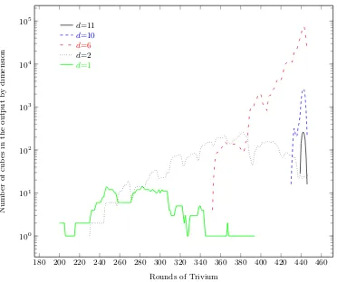
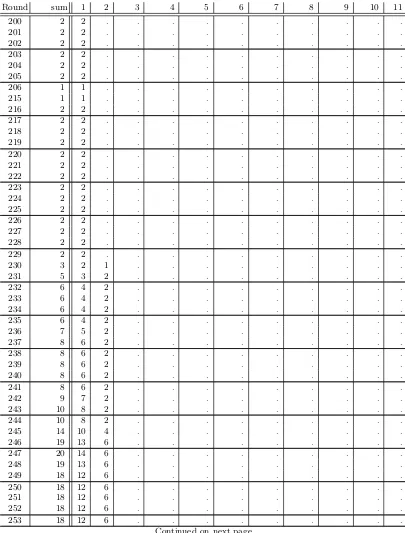
number of possible monomials is bounded from above by 2|K|+|V|. In the case of Trivium, we have 2160. To this aim, we have a closer look at the actual dimension of cubes, cf. figure 6. Here, we see the same cubes as in figure 3 but do distinguish them by their dimension. To keep figure 6
readable, we did restrict to dimensions 1,2,6,10 and 11. A list ofall cubes by dimension is given in table3. First we note that some cube dimensions only occur after a particular round. For example, we do not have cubes of dimension 10 before round 430 (dimension 11: round 439). This finding is in line with the overall definition of Trivium: All state bits are initialized with polynomials of degree -1, 0 or 1. The output function of Trivium does not change this as it only contains addition, no multiplication. However, the update function of Trivium for each inidividual state contains exactly one multiplication of two previously computed state bits. Hence, the overall degree of the corresponding polynomial will most likely increase here and give rise to new (potential) cubes. In addition we notice that we do not have any cubes of dimension 1 after round 394 and that there are rounds without cubes of dimension 1 from round 362 onwards. To tackle this question, we have a closer look how cubes develop in the following section.
Regarding the number of monomials we see the corresponding plot is far smoother and we have at least an order of magnitude more monomials than cubes for a given round. Even though, giving a closed formula or even extrapolating is difficult enough.
6.2 Life-cycle of a Cube
180 200 220 240 260 280 300 320 340 360 380 400 420 440 460 100
101 102 103 104 105
Rounds of Trivium
Num
b
er
of
cub
es
in
the
output
b
y
dimension
d=1
d=2
d=6
d=10
d=11
Fig. 6. Number of cubes of dimension d in the output of Trivium, plotted per dimension d = 1,2,6,10,11 against the number of rounds.
1. Non-existence 2. Creation 3. Destruction
In phase 1, a cubeC cannot exist as there is no monomial that contains the corresponding variables from the set of IV variablesV, plus exactly one variable from the set of key variablesK. As soon as this changes, we are in phase 2. Now, we have at least one monomial that is of the formxCki with
ki∈K and C⊂V. Finally, we may have a monomial of the form xCkikj with 0≤i, j <80, i6=j. This will destroy the cube, and we are in phase 3. Note that any monomial with at least two key variables will do to destroy the corresponding cubexC. Alternatively, we can use the definitions of section 2.3 and say that a cube is constant (one or negative) is phase 1, linear in phase 2, and a higher-order (quadratic, cubic) cube in phase 3. We illustrate this with the following example.
Example 13. Let K := {a, b, c}, V := {α, β} be the sets of key and IV variables, respectively. Moreover, consider the following function f :K∪V →Bin algebraic normal form (ANF):
f(K, V) :=aα+cα+cαβ+bcαβ+a