Daniel J. Bernstein1,3, Jeroen Doumen2, Tanja Lange3, and Jan-Jaap Oosterwijk3
1 Department of Computer Science
University of Illinois at Chicago, Chicago, IL 60607–7053, USA [email protected]
2 Irdeto, CTO Research Group, Taurus Avenue 105, 2132 LS, Hoofddorp, The
Netherlands [email protected]
3 Department of Mathematics and Computer Science
Technische Universiteit Eindhoven, P.O. Box 513, 5600 MB Eindhoven, The Netherlands
[email protected],[email protected]
Abstract. Batch signature verification detects whether a batch of sig-natures contains any forgeries. Batch forgery identification pinpoints the location of each forgery. Existing forgery-identification schemes vary in their strategies for selecting subbatches to verify (individual checks, bi-nary search, combinatorial designs, etc.) and in their strategies for veri-fying subbatches. This paper exploits synergies between these two levels of strategies, reducing the cost of batch forgery identification for elliptic-curve signatures.
Keywords: Signatures, batch verification, elliptic curves, scalar multi-plication
1
Introduction
Our goal in this paper is to minimize the cost of elliptic-curve signature verifica-tion. As an illustration of our results, one of our algorithms verifies a sequence of 64 elliptic-curve signatures (from 64 different signers) at a 2128 security level using
– a total of 0.9·64·128 additions if all signatures turn out to be valid, – a total of 1.3·64·128 additions if 2 signatures turn out to be invalid, – a total of 2.3·64·128 additions if 10 signatures turn out to be invalid, and – a total of 3.6·64·128 additions if all 64 signatures turn out to be invalid.
For comparison, we use a total of 2.8·64·128 additions to separately verify the same 64 signatures.
We emphasize that our algorithms pinpoint the forgeries. These algorithms are not merely “batch signature verification” algorithms, saying yes if and only if all of the signatures are valid; these algorithms are “batch forgery identification” algorithms, telling the user separately for each signature whether that signature is valid. The main challenge we address is to locate each forgery as efficiently as possible.
Cost metric. We systematically report the costs of our algorithms in group operations: the total number of elliptic-curve doublings, additions, and subtrac-tions. For conciseness we write “additions” rather than “group operations”, but readers evaluating costs in more detail should be aware that doublings are less ex-pensive than additions in typical elliptic-curve coordinate systems, that “mixed additions” save time, etc.
We also caution the reader that elliptic-curve computations often involve sig-nificant overhead beyond group operations. For example, the CHES 2011 elliptic-curve-signatures paper [4] by Bernstein, Duif, Lange, Schwabe, and Yang reports quite noticeable time, even after various speedups, for decompressing points and for manipulating a priority queue of scalars. We would expect our algorithms to use the same amount of time for decompression and less time for manipulat-ing scalars, but properly verifymanipulat-ing these predictions would require an optimized assembly-language implementation at the level of [4].
Our verification algorithms are randomized. Performance depends somewhat on these random choices, but our experiments indicate that the variance in performance (for any particular number of forgeries) is quite small.
The total cost of separately verifyingnsignatures at a 2b security level scales linearly in n and almost linearly in b: it has the form αnb where α is indepen-dent of nand nearly independent of b. This paper’s batch-forgery-identification algorithms useαnbadditions whereα is a more complicated function ofn,b, the number of forgeries, and various algorithm parameters. We systematically report the number of additions in the form αnb, as illustrated by the 0.9nb example above with n= 64 and b= 128.
Choice of signature system. We focus on the EdDSA signature system pro-posed in [4]. This system is a tweaked version of the classic Schnorr signature system [35]; one of the tweaks allows much faster batch verification.
In EdDSA, verifying a signature (R, S) on a message M under a public key
A means verifying an equation of the form SB =R+hA. Here B is a standard elliptic-curve point, R and A are elliptic-curve points, S is a scalar, and the scalar h is a hash of R, A, andM.
For comparison, in Schnorr’s system, the signature is (h, S) rather than (R, S). The verifier recomputesR=SB−hAand then checks that the hash matchesh. This is not compatible with our verification algorithms: our algorithms require
R as input.
An analogous tweak for DSA (and the general idea of sending R instead of
in [23]. We prefer Schnorr to ECDSA (and prefer EdDSA to tweaked ECDSA) for several reasons: Schnorr eliminates inversions, for example, and is resilient to hash-function collisions.
For elliptic-curve signatures at a 2b security level it is standard practice to use about 2b bits for hashes, scalars, and field elements, and to compress points to single coordinates. EdDSA and Schnorr’s system then have the same signature size, about 4bbits. Additions require uncompressed points, so the standard way to verify a signature in Schnorr’s system is to decompress the public key A, compute SB −hA, compress the result to obtain R, compute the hash, and check for a match with h. We emphasize that the same operations, in a different order, verify a signature in EdDSA: compute the hashh, decompress the public key A, compute SB −hA, compress the result, and check for a match with
R. The advantage of EdDSA is that it allows further choices for the verifier: fast batch verification, as discussed in [4], and fast batch forgery identification, as discussed in this paper. These algorithms require decompression of both A
andRfor each signature, but amply compensate for the extra decompression (an extra square-root computation) by eliminating a large fraction of the subsequent elliptic-curve operations.
One can merge EdDSA with Schnorr’s system, simultaneously allowing sig-natures of the form (h, S) and signatures of the form (R, S). The first step in verifying an EdDSA signature computes, as a side effect, a Schnorr signature for the same message; similarly, one of the (later) steps in verifying a Schnorr signature computes, as a side effect, an EdDSA signature. It is not commonly appreciated that Schnorr’s system actually allows hashes as short as b bits (as pointed out by Schnorr), reducing a signature to about 3b bits; users then have the flexibility to convert signatures from EdDSA format to Schnorr format to save space, and to convert signatures from Schnorr format to EdDSA format for fast batch forgery identification. One can of course also save decompression time by transmitting uncompressed signatures and uncompressed public keys.
Pairing-based signatures allow shorter signatures, about 2b bits, but pairing-based verification is an order of magnitude slower than elliptic-curve verification. Consider, for example, [21, Figures 1(a), 2(a), 3(a), 4(a)]: batch verification of pairing-based signatures with b = 80 costs about 214 field multiplications per signature, i.e., about 200nb field multiplications. This is the cost in the best case, when there are no forgeries; the cost increases rapidly with the number of forgeries. For comparison, Hisil et al. showed in [12] how to reduce the cost of an elliptic-curve addition to at most 8 field multiplications; we never use more than 4nb additions, i.e., 32nb field multiplications.
fac-tor between 2 and 3 compared to the simplest binary methods of computing
`P +mQ. There are also many lower-level speedups inside elliptic-curve addi-tions, field arithmetic, etc., but these speedups have no effect on the number-of-additions metric used for the rest of this paper.
There are, as mentioned above, some papers proposing batch verification of elliptic-curve signatures. The central idea is to check that several quantities
V1 = R1 +h1A1 −S1B, V2 = R2 + h2A2 −S2B, etc. are all 0 by checking whether a random linear combination
V =z1R1+z2R2+· · ·+ (z1h1)A1+ (z2h2)A2+· · · −(z1S1+z2S2+· · ·)B is 0. If the verifier chooses the “randomizers” z1, z2, . . . as independent uniform random 128-bit integers then this test cannot be fooled with probability above 2−128. We emphasize the importance of including these randomizers; in Section 2 we explain how to break the non-randomized batch-verification system from a very recent paper.
This linear-combination idea was proposed in [23] for (tweaked) DSA, in the simpler (and faster but obviously less useful) case of verifying multiple signatures of the same user, i.e. A1 = A2 = · · ·. The speedup in [23] was only a small constant for high security levels, because [23] computedV using only very simple techniques for multi-scalar multiplication, but [4] showed that the Bos–Coster multi-scalar multiplication method produced a much larger speedup. It is easy to see that the speedup here is asymptotically Θ(lgn) for a batch of nsignatures. The first paper to point out a non-constant speedup was [2] by Bellare, Garay, and Rabin, using a different technique that does not appear to be competitive with advanced multi-scalar multiplication methods.
What is missing from all of these papers is an efficient way to handle forgeries. Consider, for example, the following quote from [4]:
If verification fails then there must be at least one invalid signature. We then fall back to verifying each signature separately. There are several techniques to identify a small number of invalid signatures in a batch, but all known techniques become slower than separate verification as the number of invalid signatures increases; separate verification provides the best defense against denial-of-service attacks.
This strategy means that an attacker sending a low volume of forgeries, enough to have one forgery in each batch, causes a severe slowdown in the software from [4]: each signature ends up being verified separately. It is of course desirable to reduce this damage, if that can be done without compromising performance under heavier denial-of-service floods; what is most desirable is to simultaneously reduce the cost of handling a few forgeries, the cost of handling many forgeries, and every case in between.
becomes slower than separate verification as the number of forgeries increases; however, this algorithm is the foundation for several improved algorithms dis-cussed below.
If one measures algorithm speed by simply counting the number of batch verifications then the binary-splitting method seems quite fast, identifying each forgery in lgn batch verifications wheren is the batch size; this is optimal for a single forgery, and diverges only slowly from optimality as the number of forgeries grows. However, the number of batch verifications is not a good measure for the actual amount of time needed to identify the forgeries. Not all verifications require the same amount of time: a larger batch takes longer. Counting additions is a much more realistic cost measure and shows that the binary-splitting method of [25] is actually quite slow.
Pastuszak, Pieprzyk, and Seberry in [26] considered the possibility of non-adaptively choosing subbatches to verify. All available evidence suggests that this non-adaptivity restriction compromises performance even when the number of forgeries is somehow known in advance, and it certainly does not improve perfor-mance. Furthermore, non-adaptivity is clearly a disaster when the approximate number of forgeries is not known in advance. We therefore focus on the more flexible adaptive case.
Zaverucha and Stinson in [39] pointed out that there was already a long lit-erature on the number of tests required by adaptive and non-adaptive “group testing” algorithms. Aside from terminology, a “group testing” algorithm is pre-cisely a forgery-identification algorithm built on top of batch verification; in particular, both [25] and [26] fit into this framework. However, the following papers (some of which predate [39]) do not fit into this framework.
Law and Matt in [18] were the first to point out, in the context of pairing-based signatures, that batch verification is providing more information than a simple “yes” or “no”. The most important idea, transported to the elliptic-curve case discussed in this paper, is that one can reuse the randomizers z1, . . . , zn from V = z1V1 +· · ·+znVn. If V 6= 0 then the binary-splitting method begins with a half-size multi-scalar multiplication to compute a left-half sum z1V1 +
· · ·+zn/2Vn/2; and then the right-half sumzn/2+1Vn/2+1+· · ·+znVn is trivially computed with a single subtraction, rather than another half-size multi-scalar multiplication.
Law and Matt also suggested computing V0 =z1V1+ 2z2V2+· · ·+nznVn. If there is just one invalid signature, sayVi 6= 0, thenV0 =iV, and one can compute
i inO(√n) additions by the baby-step-giant-step method. Further development of this approach appears in [18], [20], and [21].
2
On the importance of being random
The paper [16] by Karati, Das, Roychowdhury, Bellur, Bhattacharya, and Iyer, appearing at Africacrypt 2012 earlier this year, proposed a scheme for batch verification of ECDSA signatures. This section shows that the scheme is insecure. The main problem is that the scheme does not randomize the linear combination being verified.
ECDSA. The basic ECDSA signature scheme works as follows. The system parameters are a prime `, a generator B of an order-` group hBi, and a cryp-tographic hash function H. The secret key of a user is a random integer a in [1, `]; the user’s public key is A =aB. The group is a subgroup of the set ofFp -rational points on an elliptic curve given in Weierstrass formy2 =x3+c4x+c6 for c4, c6 ∈Fp. An affine point is a tuple P = (x(P), y(P)) satisfying the curve equation; the negative of this point is −P = (x(P),−y(P)). The curve consists of the affine points and the point at infinity P∞, which is the neutral element of the group of points.
A signature on messageM under public key A is a tuple (r, s) such that the
x-coordinate of (H(M)/s)B+ (r/s)A is congruent to r modulo `. The standard approach to verification is to compute R = (H(M)/s)B+ (r/s)A and to check that x(R) is congruent to r modulo `.
The scheme from [16] for batch ECDSA verification. The batch verifi-cation scheme described in [16] verifies signatures (ri, si) on messages Mi and public keysAi for 1≤i≤nby reconstructing Ri from ri and checking whether Pn
i=1Ri equals ( Pn
i=1H(Mi)/si)B+ Pn
i=1(ri/si)Ai.
The obvious approach to reconstructing Ri from ri is to first compute x(Ri) from x(Ri) mod` = ri and then compute y(Ri) from the curve equation. The first step is straightforward in the common case that ` ≈ p: there is almost always a unique integer x(Ri) ∈ {0,1, . . . , p−1} satisfying x(Ri) mod` = ri. The second step is more difficult: it seems to require a square-root computation, and furthermore can at best determine ±y(Ri); in a batch of n signatures one needs to guess as many as 2n combinations of signs. This implies that the batches need to be chosen small; in [16] the maximum batch size considered is 8. The paper puts the main effort into developing new techniques for computing P
Ri from the x-coordinates in a more efficient manner and reports a good speed-up factor compared to individual verification.
First attack. A batch signature system is broken if invalid signatures pass as valid. The easiest way to break the above scheme is to submit (r, s) as a signature on a target messageM under a target public keyAand also (r,−s) as a signature on the same message under the same public key, where r is any x-coordinate of a curve point. The verification algorithm reconstructs two points R,−R having
x-coordinater, and then the contributions of these signatures cancel out in both sums:
This attack relies on the fact that r does not pinpoint a unique R: it can be expanded to R and to −R.
These forgeries are easy to detect once the system is altered to check for them. Excluding a sum of P∞ is not adequate if the batch includes other signatures along with these two forgeries, but checking for repeated r values is adequate. However, as we will see in a moment, there are other attacks on the scheme that are much more difficult to detect.
Second attack. Assume that the attacker knows the secret key a2 for a public key A2. The following attack convinces the verifier to accept a signature on any target message M1 under any target public key A1, along with a signature on
M2 under A2.
The attacker picks a random k1, and computes R1 = k1B and r1 = x(R1) as in proper signature generation. He then picks a random s1 and computes
R2 = (r1/s1)A1, r2 = x(R2), and s2 = (H(M2) + r2a2)/(k1 − H(M1)/s1); the denominators are nonzero with overwhelming probability. The attacker then submits (r1, s1) as signature on M1 from A1 and (r2, s2) as signature on M2 from A2 to the batch system.
The verifier now reconstructs the same R1 and R2, and computes R1 +R2 and (H(M1)/s1 +H(M2)/s2)B+ (r1/s1)A1 + (r2/s2)A2, both of which equal
k1B+ (r1/s1)A1. These forgeries thus pass verification, even though neither of them is valid individually and the attacker does not know the secret key for A1. The forgeries also work if they are batched together with other signatures in the same verification.
As far as we can tell, the most efficient way to distinguish (r1, s1) and (r2, s2) from properly formed signatures is to verify them separately. This trivial batch-verification scheme is obviously secure but also sacrifices all of the speedup re-ported in [16].
Consequences. These attacks show that the scheme considered in [16] is inse-cure. The second attack would work even if the ECDSA signature system were replaced by a signature system such as EdDSA that transmits R instead of r, removing the±Rambiguity. The second attack shows that it is important to use randomness in the tests: to introduce n sufficiently random integers zi to scale the equations and verify Pn
i=1ziRi = (P n
i=1ziH(Mi)/si)B+P n
i=1(ziri/si)Ai instead.
Randomizers were used in the original batch signature scheme introduced by Naccache, M’Ra¨ıhi, Vaudenay, and Raphaeli in [23]. There is no discussion of randomizers in [16], and in particular no explanation of why the randomiz-ers were omitted in [16], but it is clear that computing Pn
i=1ziRi would take much longer than computing Pn
i=1Ri, and it is even harder to compute its x -coordinate from the ri without square-root computations to recover each point
3
High level: Binary search
This section presents a family of algorithms for verifying a batch of n EdDSA signatures. We begin with a simple binary-search algorithm and then discuss several variants of the algorithm.
These algorithms rely on multi-scalar multiplication as a lower-level subrou-tine. Section 4 presents several multi-scalar multiplication algorithms usable in this context, pointing out new synergies between these two levels of algorithms. Section 5 analyzes the overall algorithm cost and reports the results of computer experiments with particular algorithm parameters.
For simplicity we assume that the batch size n is a power of 2. Other batch sizes can be split into power-of-2 batch sizes, or handled directly by straightfor-ward generalizations of the algorithms here.
We also assume for simplicity that B has prime order `, and that all input points Ri, Ai are known in advance to be in the group generated by B. For elliptic-curve groups with small cofactors the usual way to ensure this is to multiply all input points by the cofactor, such as the cofactor 8 in [3] and [4]. A closer look shows that this multiplication can safely be suppressed in the context of signature verification, but since the multiplication has very low cost we skip further discussion.
Randomizers. All of our algorithms use the randomizers zi discussed in Sec-tions 1 and 2. As precomputation we choose z1, z2, . . . , zn independently and uniformly at random from the set 1,2,3, . . . ,2b , where b is the security level. There are several reasonable ways to do this: for example, generate a uniform randomb-bit integer and add 1, or generate a uniform randomb-bit integer and replace 0 with 2b.
Of course, it is also safe to simply generate zi as a uniform random b-bit integer, disregarding the negligible chance that zi = 0; but this requires minor technical modifications to the security guarantees stated below, so we prefer to require zi 6= 0. It is also safe to simulate random numbers as outputs of a strong stream cipher using a long-term random secret key; this is helpful on platforms where generating randomness is expensive. Rather than maintaining stream-cipher state (e.g., the counter in the AES-CTR stream cipher) one can safely encrypt a collision-resistant hash of the input batch.
We also precompute integersh1, h2, . . . , hn as the standard (system-specified) hashes of (R1, A1, M1),(R2, A2, M2), . . . ,(Rn, An, Mn) respectively. By defini-tion theith signature is valid ifSiB=Ri+hiAi, and a forgery ifSiB 6=Ri+hiAi. Leaf randomizers. In this section we define Vi = zi(Ri+hiAi−SiB). Note the inclusion ofzi here, deviating from Section 1. This is not merely a change of notation: to verify a single signature (when this is required), our algorithm com-putes this Vi, whereas the standard verification approach from [4] is to compute
SiB−hiAi. Note that signature i is valid if and only if Vi = 0.
The standard approach would seem at first glance to be more efficient: com-puting SiB−hiAi involves two full-size (2b-bit) scalars Si, hi, while computing
V
dddddddddddddddddd
dddddddddddddd
V1,8
jjjjjjjjjj
jjjj V9,16
jjjjjjjjjj jjjj
V1,4
tttttt
V5,8
tttttt
V9,12
tttttt
V13,16
tttttt
V1,2
V3,4
V5,6
V7,8
V9,10
V11,12
V13,14
V15,16
V1 V2 V3 V4 V5 V6 V7 V8 V9 V10 V11 V12 V13 V14 V15 V16
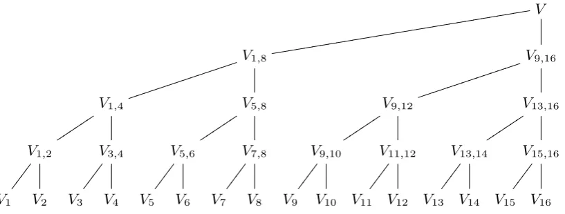
Fig. 3.1. Tree of sums of randomized leaves V1, V2, . . . , Vn for n= 16.
and a half-size scalar zi, for a total of 25% more scalar bits. However, the cost of multi-scalar multiplication (see Section 4) is affected much more by the max-imum number of scalar bits than by the total number of scalar bits; the cost of computing Vi turns out to be only slightly higher than the cost of computing
SiB−hiAi. This slight extra expense pays off in subsequent steps of the batch algorithm, as discussed below.
Shared randomizers. Starting from these randomized quantities V1, . . . , Vn we draw a binary tree as illustrated in Figure 3.1, with V1,2 = V1 + V2 and
V3,4 =V3+V4 and so on at the second level,V1,4 =V1,2+V3,4 and so on at the third level, etc. In general we write Vj,k for the sum Pj≤i≤kVi of leaf nodes. If all of the signatures at positions j, j+ 1, . . . , k are valid then Vj,k = 0, while if any of the signatures are invalid then with overwhelming probability Vj,k 6= 0. The root node V1,n at the top represents the randomized signature verification of the entire batch; we denote this sum by V as a shorthand.
The set of tree nodes actually computed by the algorithm is determined adap-tively; see below.
nodes). There are n−1 non-leaf nodes, so a randomizer sequence is bad with probability at most (n−1)/2b.
The basic batch-forgery-identification algorithm.The following algorithm takes as input public keysA1, A2, . . . , An, signatures (R1, S1), . . . ,(Rn, Sn), pre-computed hashes h1, h2, . . . , hn, and precomputed randomizers z1, z2, . . . , zn. The algorithm also takes an optional input V; this is used when the algorithm calls itself recursively in Step 5.
The algorithm provides two outputs: first,V, whether or not V was provided as input; second, ann-bit string (b1, b2, . . . , bn). With overwhelming probability
bi = 1 if and only if signaturei is valid. The algorithm has six steps:
1. Batch verification: Compute V = P
izi(Ri +hiAi−SiB), if V was not provided as input. Output V. If V = 0, output n bits (1,1, . . . ,1) and stop. 2. Forgery rejection: Ifn= 1, output (0) and stop. (At this point V 6= 0, so
the signature is invalid.)
3. Left subtree: Apply the same algorithm recursively to A1, A2, . . . , An/2; (R1, S1), . . . ,(Rn/2, Sn/2); h1, . . . , hn/2; and z1, . . . , zn/2; obtaining outputs
V1,n/2 and (b1, . . . , bn/2).
4. Right root:IfV1,n/2 = 0, setVn/2+1,n =V. IfV1,n/2 =V, setVn/2+1,n = 0. Otherwise compute Vn/2+1,n =V −V1,n/2.
5. Right subtree: Apply the same algorithm recursively to An/2+1, . . . , An; (Rn/2+1, Sn/2+1), . . . ,(Rn, Sn);hn/2+1, . . . , hn;zn/2+1, . . . , zn; andVn/2+1,n; obtaining outputs Vn/2+1,n and (bn/2+1, . . . , bn).
6. Final output: Output (b1, . . . , bn).
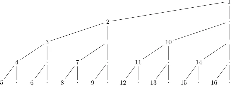
This algorithm is optimistic, hoping that there are no forgeries: Step 1 finishes the algorithm as quickly as possible in this case. See Section 4 for details of the computation in this step. The overall binary-splitting structure of this algorithm is taken from [25]. The fast computation of Vn/2+1,n in Step 4, using at most one subtraction, is taken from [18]; this is also the reason for treating V as an output and an optional input. This fast computation means that at most n
nodes require a multi-scalar multiplication in Step 1; Figure 3.2 illustrates the worst case.
Another way to organize essentially the same computation is to record a partial tree of known Vj,k values, and to very quickly update the tree whenever a forgery is discovered, in effect retroactively removing the forgery from the batch. Start the computation at the root; after computing a zero node, deduce without further computation that all descendants of the node are also zero; after computing a nonzero leaf node Vi 6= 0, replace all ancestors Vj,k by Vj,k−Vi, skipping the subtraction in the common case that Vj,k =Vi; after computing a nonzero non-leaf node, compute the left child node (and all of its descendants in order), and then simply copy this (possibly updated) node to the right child node.
Leaf randomizers, continued.In the casen= 1 this algorithm computesV1 =
1
dddddddddddddddd
ddddddddddddddddd
2
jjjjjjjjjj
jjjjjjj
.
jjjjjjjjjj
jjjjjj
3
tttttt
tt .
tttttt
ttt 10
tttttt
t .
tttttt tt
4
.
7
.
11
.
14
.
5 . 6 . 8 . 9 . 12 . 13 . 15 . 16 .
Fig. 3.2.Tests in worst case are depicted in order.
than computing S1B−h1A1. We now explain the compensating advantage of computing V1.
Consider a batch of two signatures that fails batch verification. i.e., V1,2 6= 0. This algorithm computes V1 (showing whether the first signature is valid), and then deduces V2 (showing whether the second signature is valid) with at most one subtraction. For comparison, one could instead compareS1B−h1A1toR1to see whether the first signature is valid, but one then still needs to check whether the second signature is valid. One could check the second signature separately, or multiplyR1+h1A1−S1B byz1 to obtainV1 and thus V2, but simply starting with V1 is less expensive.
Early abort.This algorithm is faster than separate verification when there are not many forgeries, but as discussed in subsequent sections it becomes noticeably slower than separate verification when there are many forgeries. The gap is not very large, but we would still like to minimize it.
We thus propose (1) using the fraction of invalid signatures found so far as an estimate for the expected fraction of invalid signatures in the rest of the tree, and (2) deciding on this basis whether it is best to abort the tree structure and check individual signatures.
An attacker might try to spoil the estimate by, e.g., placing several invalid signatures at the beginning of a large batch. After those signatures the algorithm will confidently, but incorrectly, estimate that the entire batch is invalid. To prevent such attacks one can simply apply a random permutation to the sequence of signatures before applying the algorithm. (One can also imagine tracking forgery percentages long term from one batch to another, but for simplicity we handle each batch separately.)
1
dddddddddddddddd
ddddddddddddddddd
2 jjjjjjjjjj jjjjjjj . jjjjjjjjjj jjjjjjj 3 tttttt tt . tttttt ttt . tttttt ttt . tttttt ttt 4 . . . . . . .
5 . 6 . 7 8 9 . 10 11 12 13 14 15 16 .
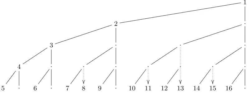
Fig. 3.3. Tests performed for n = 16 when all signatures are invalid, using the early abort. Arrows denote the test replacements and savings.
whenever a node is about to be computed. In the notation of the basic algorithm above, we dynamically choose between
– optimism: computing V, and then, ifV 6= 0, computingV1,n/2 and deducing
Vn/2+1,n =V −V1,n/2; or
– pessimism: computing V1,n/2 and Vn/2+1,n, and then deducingV =V1,n/2+
Vn/2+1,n.
If V is provided as input then optimism is better. If V is not provided as input then we use (1 − p)n as an estimate of the chance that V = 0, where p is the fraction of invalid signatures found so far (or 0 at the beginning of the algorithm), and then compare the expected costs of optimism and pessimism, using straightforward models of the costs of computing V, V1,n/2, Vn/2+1,n.
When there are few forgeries, this approach performs the same computations as the basic algorithm. When there are many forgeries, this approach rapidly con-verges on checking each signature separately, as shown in Figure 3.3. Compared to the previous worst case, where we computed the top node of each vertical branch, we now only need to compute the top nodes of the main left diagonal branch. In all other vertical branches, the leaf node is computed directly. (One can do marginally better in this extreme case by immediately updating p after discovering V1,16 6= 0: there must be a forgery somewhere, even though it has not been located yet.)
directly toV17,20. If the fraction of invalid signatures remains stable then we will check these 16 signatures as 4 batches of 4 signatures each. We then decide anew how to check the next 32 signatures.
Smaller randomizers. Large randomizers zi are critical for detecting multi-forgeries, as discussed in Section 2, but this does not mean that large randomizers are required at each step of the tree. An alternative approach is to use one sequence of large randomizers at the root, and to use a second sequence of much smaller randomizers, say 20 bits each, for the subsequent levels of the tree.
This approach slightly speeds up multi-scalar multiplication at non-root nodes. However, this approach also has several costs. First, the right child of the root node is no longer obtained for free. Second, the sharing described in Section 4 begins only at the children of the root node, not at the root node itself. Third, an attacker can fool the smaller randomizers with noticeable probability, on the scale of 2−20, so after identifying forgeries using the smaller randomizers one must recompute the corresponding portion of the root node. If this root-node update shows that any forgeries remain then one must choose a new sequence of smaller randomizers and try the computation again on the remaining signatures.
4
Low level: Trees of optional multi-scalar multiplications
This section looks more closely at the first step of the algorithm of Section 3: namely, batch verification, i.e., computing a linear combination
V =z1R1+· · ·+znRn+ (z1h1)A1+· · ·+ (znhn)An−(z1S1+· · ·+znSn)B of known elliptic-curve points R1, . . . , Rn, A1, . . . , An, B. If V 6= 0 then the al-gorithm calls itself recursively and computes a smaller linear combination
V1,m=z1R1+· · ·+zmRm+ (z1h1)A1+· · ·+ (zmhm)Am−(z1S1+· · ·+zmSm)B with m=n/2.
The computation of V by itself is a standard (2n+ 1)-scalar-multiplication problem. The only mildly uncommon feature of this problem is that the scalars have variable size, typicallyn128-bit scalars (thezi’s) andn+ 1 256-bit scalars; but typical scalar-multiplication algorithms can trivially take advantage of the shorter scalars. Similarly, the computation ofV1,mby itself is a standard (2m +1)-scalar-multiplication problem.
Quite nonstandard, however, is the multi-scalar-multiplication problem that we actually face: computing V and then perhaps computing V1,m. If we knew that we wanted to compute bothV andV1,mthen the obvious approach would be two separate half-size computations, one forV1,m and one forVm+1,n =V−V1,m; but we do not know this in advance. IfV turns out to be 0 then we will not need
V1,m and Vm+1,n, and a single full-size computation of V will be more efficient than two separate half-size computations.
many intermediate results useful for computing V1,m. The same idea can easily be pushed to further levels: for example, computing V, then optionally V1,m, then optionally V1,bm/2c and optionally Vm+1,m+1+b(n−m)/2c.
Overlap in the Bos–Coster approach. As an illustration of what does not seem to work very well in this context, consider the Bos–Coster algorithm re-ported in [8, Section 4]. This algorithm computes a1P1 + a2P2 +a3P3 +· · ·, wherea1 ≥a2 ≥a3 ≥ · · ·, by recursively computing (a1−a2)P1+a2(P1+P2) +
a3P3+· · ·. This algorithm was used in [4] to compute V.
The first few additions performed in the Bos–Coster algorithm depend only on the largest scalars. If we permute signatures so that z1h1 ≥z2h2 ≥ · · ·, and handlez1S1+· · ·+znSnseparately, then the first≈madditions in the algorithm will involve only A1, . . . , Am, and will thus be the same as the first additions involved in computing V1,m. However, this is only a slight speedup.
Overlap in the Straus approach. As a better example, consider the Straus algorithm [37], often miscredited to Shamir. This algorithm computes a1P1+
a2P2 + · · · + anPn by recursively computing ba1/2ccP1 + ba2/2ccP2 + · · · +
ban/2ccPn, doublingctimes, and then adding the precomputed quantity (a1 mod 2c)P1+ (a2 mod 2c)P2+· · ·+ (an mod 2c)Pn. Here 2c is a radix chosen by the algorithm; for example, it is reasonable to takec= 5 for 256-bit scalars. We skip discussion of standard speedups such as signed digits.
This algorithm scales poorly to large values of n (because it involves too much precomputation, even for c = 1), but a standard variant scales well to large values of n: at the last step one instead adds the separate precomputed quantities (a1 mod 2c)P1, (a2 mod 2c)P2, etc.
Evidently one can reuse these precomputed quantities for a subsequent multi-scalar multiplication involving P1, . . . , Pm with the same choice of c. Further-more, if the precomputed quantities are added from left to right in each step, then one of the intermediate results is exactly (a1 mod 2c)P1+· · ·+ (am mod 2c)Pm. This drastically reduces the cost of computing a1P1 +· · ·+amPm when m is large: each step of the recursion drops from cost c+ m (c doublings and m
additions) down to justc+ 1.
The same overlap applies immediately to a1P1 + · · ·+abm/2cPbm/2c. Even better, if we change the order to add precomputed quantities, recursively adding the P1, . . . , Pm part and the Pm+1, . . . , Pn part, then the same overlap applies not just to left descendants but to arbitrary descendants.
Overlap in the Pippenger approach.As a more advanced example, consider Pippenger’s multi-scalar-multiplication method. This method was published in [28] almost forty years ago; various special cases of the method were subsequently reinvented and published in the papers [6] and [19] and continue to be frequently miscredited to those papers. We comment that the patent accompanying [6] (U.S. patent 5299262) expired this year.
essentially all sequences of scalars; see generally [30]. Of course, this does not imply that Pippenger’s method is optimal for the problem of computing V and then perhaps V1,m, but inspecting the details shows that Pippenger’s approach does allow considerable savings in computing V1,m.
The following special case of Pippenger’s algorithm has similar performance to the Bos–Coster method and is adequate to illustrate the idea. Choose a radix 2c as above, and proceed as in Straus’s algorithm, but replace the last step with the following computation. Sort the points P1, P2, . . . , Pn into 2c buckets according to the values a1 mod 2c, a2 mod 2c, . . . , an mod 2c. Discard bucket 0 and add the points in the remaining buckets, obtaining sumsS1, . . . , S2c−1. Now compute
(a1 mod 2c)P1+· · ·+ (an mod 2c)Pn=S1+ 2S2+· · ·+ (2c−1)S2c−1 as the sum of the intermediate quantities S2c−1, S2c−1 +S2c−2, . . ., S2c−1 +
S2c−2+· · ·+S1.
Observe that computinga1P1+· · ·+amPm in the same way, using the same value of c, puts P1, P2, . . . , Pm into exactly the same buckets. If for the a1P1+
· · ·+anPn computation we are careful to add points in each bucket from left to right then the intermediate result after P1, P2, . . . , Pm will be exactly the sum relevant to a1P1 +· · · +amPm. For typical parameters there are several points in each bucket, so this approach is several times faster than a standard computation of a1P1 +· · ·+amPm. As before, it is even better to change the order to add points in each bucket, recursively adding the points that come from
P1, P2, . . . , Pm and the points that come from Pm+1, . . . , Pn.
Handling the base point.These modified versions of the Straus and Pippenger methods apply directly to
z1R1+ (z1h1)A1+· · ·+znRn+ (znhn)An
but do not apply directly to (z1S1+· · ·+znSn)B, the last component ofV. The simplest way to handle these multiples of B is to compute them sepa-rately. Because B is a fixed base point, one can afford a precomputed table of, e.g., B,2B,3B, . . . ,(2c−1)B and 2cB,2·2cB,3·2cB, . . . ,(2c−1)·2cB and so on. Computing any desired multiple of B then takes fewer than 1/c additions for each bit of the scalar, a very small cost compared to the other computations discussed here.
5
Analysis
This section analyzes the cost of identifying all of the forgeries amongn elliptic-curve signatures at a 2b security level. Full-size scalars such as hi, Si, zihi mod
`, ziSi mod` then have 2b bits as discussed in Section 1, while the randomizers
zi have bbits.
Separate signature verification.Solinas’ widely used Joint Sparse Form [36] handles a double-scalar multiplication hiAi −SiB using 2b doublings and on average b additions, for a total cost of 3nb to handlen signatures.
Straus’s method is asymptotically more efficient, handling n signatures at cost (2 +o(1))nb as b → ∞. Straus’s method involves approximately 2b dou-blings; every cdoublings are followed by 2 additions, and on average a fraction 1/2c of the additions are skippable additions of 0. The additions rely on an initial computation of 2A1,3A1, . . . ,(2c−1)A1, which costs 2c−2, and a free precompu-tation of 2B,3B, . . . ,(2c−1)B. The total cost fornsignatures is approximately (2b+ (1−1/2c)(2/c)2b+ 2c−2)n. One can balance the terms (1−1/2c)(4/c)b
and 2c −2 by taking c close to 2 + lgb−lg lgb; the total cost is then roughly (2 + 8/lgb)nb.
Our separate3.py software uses Straus’s method with c = 4 and with two standard speedups, namely signed digits and sliding windows. This software uses, on average, fewer than 2.8nb additions for b = 128. There is a small variance: 2.75nband 2.82nb are not unusual. We would expect more detailed optimization here, in particular using more precomputed multiples of B, to beat 2.7nb. Batch verification.All of our batch-forgery-identification algorithms start with batch verification, computingV. If there are no forgeries — no attackers attempt-ing to fool the receiver or deny service — then this is the end of the computation. Straus’s algorithm computes V with 2b doublings as above, approximately
n(b/c) additions for parts of ziRi, approximately n(2b/c) additions for parts of (zihi)Ai, and negligible cost for B. The additions rely on initial computations costing 2n(2c−2). The total cost is approximately (2/n+ 3/c+ 2(2c−2)/b)nb. Ifc is chosen close to lg(1.5b)−lg lgbthen this cost is roughly (2/n+ 6/lgb)nb. Our straus6.py software, with b= 128 and c = 5, uses 1.15nb additions for
n = 16; 0.98nb additions for n = 16; 0.90nb additions for n = 32; and 0.86nb
additions for n= 64.
We also experimented with the Bos–Coster algorithm (boscoster2.py) and did some preliminary analysis of Pippenger’s algorithm. Compared to Straus’s algorithm, we obtained better batch-verification speeds with the Bos–Coster al-gorithm (e.g., cost 0.55nbforn= 64 andb= 128) and we expect to obtain better batch-verification speeds with Pippenger’s algorithm. Asymptotically the Bos– Coster algorithm costsO(nb/lgn) and Pippenger’s algorithm costsO(nb/lgnb). However, we decided to focus on Straus’s algorithm for our experiments because Straus’s algorithm allows much better reuse of intermediate results inside batch forgery identification.
Batch forgery identification.For concreteness we focus on the overlap inside Straus’s algorithm inside binary search using shared randomizers (including leaf randomizers), without early aborts. After the root node (i.e., the batch verifi-cation discussed above), reuse of intermediate results reduces each subsequent multi-scalar multiplication to approximately 2b doublings and 4b/c additions.
0.8 1.0 1.2 1.4 1.6 1.8 2.0 2.2 2.4 2.6 2.8 3.0 3.2 3.4 3.6 3.8
0 1 2 3 4 5 6 7 8
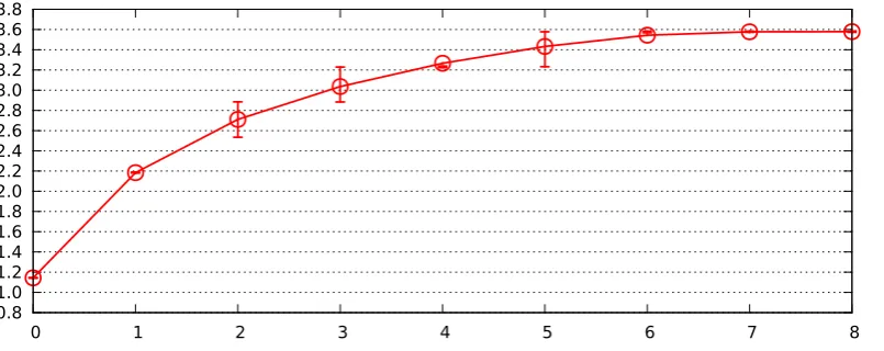
Fig. 5.1.Observed costαnbof identifying forgeries amongn= 8 signatures forb= 128. Horizontal axis is number of forgeries. Vertical axis is α. Each circle indicates average cost over 101 experiments; error bars indicate quartiles.
(2 +o(1))bafterO(nb/lgb) for the root, so the total cost is at most (2 +o(1))nb, just like separate signature verification. If a positive constant fraction of the signatures are valid then the number of nodes required is a constant factor below
nand this strategy is a constant factor faster than separate signature verification; if the number of forgeries drops then this strategy becomes a logarithmic factor faster than separate signature verification.
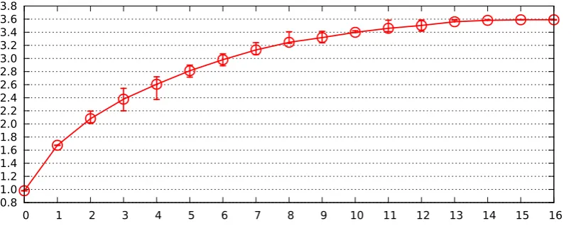
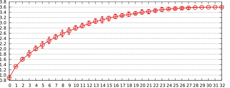
For constant b, such as b= 128, the picture is more complicated. Each com-puted non-root node has similar cost to a separate signature verification (in fact slightly lower cost), but the root node adds a significant extra cost, so this al-gorithm becomes noticeably slower than separate signature verification as the number of forgeries increases. Our straus6.py computer experiments indicate that the cutoff is around n/3 forgeries forb= 128. See Figures 5.1, 5.2, and 5.3.
References
[1] — (no editor),17th annual symposium on foundations of computer science, IEEE Computer Society, Long Beach, California, 1976. MR 56:1766. See [28].
[2] Mihir Bellare, Juan A. Garay, Tal Rabin,Fast batch verification for modular ex-ponentiation and digital signatures, in Eurocrypt ’98 [24] (1998), 236–250. URL:
http://cseweb.ucsd.edu/~mihir/papers/batch.html. Citations in this docu-ment: §1.
[3] Daniel J. Bernstein,Curve25519: new Diffie-Hellman speed records, in PKC 2006 [38] (2006), 207–228. URL: http://cr.yp.to/papers.html#curve25519. Cita-tions in this document: §3.
[4] Daniel J. Bernstein, Niels Duif, Tanja Lange, Peter Schwabe, Bo-Yin Yang, High-speed high-security signatures, in CHES 2011 [31] (2011). URL:http://eprint. iacr.org/2011/368. Citations in this document:§1,§1,§1,§1,§1,§1,§1,§3,§3,
§4.
0.8 1.0 1.2 1.4 1.6 1.8 2.0 2.2 2.4 2.6 2.8 3.0 3.2 3.4 3.6 3.8
0 1 2 3 4 5 6 7 8 9 10 11 12 13 14 15 16
Fig. 5.2. Same as Figure 5.1 but for n= 16.
1989, proceedings, Lecture Notes in Computer Science, 435, Springer, 1990. ISBN 3-540-97317-6. MR 91b:94002. See [34].
[6] Ernest F. Brickell, Daniel M. Gordon, Kevin S. McCurley, David B. Wilson,Fast exponentiation with precomputation (extended abstract), in Eurocrypt ’92 [33] (1993), 200–207; see also newer version [7]. Citations in this document:§4,§4. [7] Ernest F. Brickell, Daniel M. Gordon, Kevin S. McCurley, David B. Wilson,Fast
exponentiation with precomputation: algorithms and lower bounds(1995); see also older version [6]. URL: http://research.microsoft.com/~dbwilson/bgmw/. [8] Peter de Rooij, Efficient exponentiation using precomputation and vector
addi-tion chains, in Eurocrypt ’94 [9] (1995), 389–399. MR 1479665. Citations in this document:§4.
[9] Alfredo De Santis (editor), Advances in cryptology — EUROCRYPT ’94, work-shop on the theory and application of cryptographic techniques, Perugia, Italy, May 9–12, 1994, proceedings, Lecture Notes in Computer Science, 950, Springer, 1995. ISBN 3-540-60176-7. MR 98h:94001. See [8], [23].
[10] Yvo Desmedt (editor), Advances in cryptology — CRYPTO ’94, 14th annual in-ternational cryptology conference, Santa Barbara, California, USA, August 21–25, 1994, proceedings, Lecture Notes in Computer Science, 839, Springer, 1994. ISBN 3-540-58333-5. See [19].
[11] Steven D. Galbraith (editor), Cryptography and coding, 11th IMA international conference, Cirencester, UK, December 18–20, 2007, proceedings, Lecture Notes in Computer Science, 4887, Springer, 2007. ISBN 978-3-540-77271-2. See [18]. [12] H¨useyin Hisil, Kenneth Koon-Ho Wong, Gary Carter, Ed Dawson, Twisted
Ed-wards curves revisited, in Asiacrypt 2008 [27] (2008), 326–343. URL: http:// eprint.iacr.org/2008/522. Citations in this document: §1.
[13] Hideki Imai, Yuliang Zheng (editors),Public key cryptography, third international workshop on practice and theory in public key cryptography, PKC 2000, Mel-bourne, Victoria, Australia, January 18–20, 2000, proceedings, Lecture Notes in Computer Science, 1751, Springer, 2000. ISBN 3-540-66967-1. See [25].
0.8 1.0 1.2 1.4 1.6 1.8 2.0 2.2 2.4 2.6 2.8 3.0 3.2 3.4 3.6 3.8
0 1 2 3 4 5 6 7 8 9 10 11 12 13 14 15 16 17 18 19 20 21 22 23 24 25 26 27 28 29 30 31 32
Fig. 5.3. Same as Figure 5.1 but for n= 32.
[15] Marc Joye, Atsuko Miyaji, Akira Otsuka (editors),Pairing-based cryptography — Pairing 2010 — 4th international conference, Yamanaka Hot Spring, Japan, De-cember 2010, proceedings, Lecture Notes in Computer Science, 6487, Springer, 2010. ISBN 978-3-642-17454-4. See [21].
[16] Sabyasachi Karati, Abhijit Das, Dipanwita Roychowdhury, Bhargav Bellur, De-bojyoti Bhattacharya, Aravind Iyer, Batch verification of ECDSA signatures, in Africacrypt 2012 [22] (2012), 1–18. Citations in this document: §2,§2,§2,§2,§2,
§2,§2,§2.
[17] Kaoru Kurosawa (editor),Information theoretic security, 4th international confer-ence, ICITS 2009, Shizuoka, Japan, December 3–6, 2009, revised selected papers, Lecture Notes in Computer Science, 5973, Springer, 2010. ISBN 978-3-642-14495-0. See [39].
[18] Laurie Law, Brian J. Matt, Finding invalid signatures in pairing-based batches, in Cirencester 2007 [11] (2007), 34–53. Citations in this document: §1,§1,§3. [19] Chae Hoon Lim, Pil Joong Lee,More flexible exponentiation with precomputation,
in Crypto ’94 [10] (1994), 95–107. Citations in this document: §4.
[20] Brian J. Matt,Identification of multiple invalid signatures in pairing-based batched signatures, in PKC 2009 [14] (2009), 337–356. Citations in this document:§1. [21] Brian J. Matt, Identification of multiple invalid pairing-based signatures in
con-strained batches, in Pairing 2010 [15] (2010), 78–95. Citations in this document:
§1,§1.
[22] Aikaterini Mitrokotsa, Serge Vaudenay (editors), Progress in cryptology — AFRICACRYPT 2012, 5th international conference on cryptology in Africa, Ifrane, Morocco, July 10-12, 2012, proceedings, Lecture Notes in Computer Sci-ence, 7374, Springer, 2012. See [16].
[23] David Naccache, David M’Ra¨ıhi, Serge Vaudenay, Dan Raphaeli,Can D.S.A. be improved? Complexity trade-offs with the digital signature standard, in Eurocrypt ’94 [9] (1994). Citations in this document:§1,§1,§1,§1,§2.
[25] Jaroslaw Pastuszak, Dariusz Michalek, Josef Pieprzyk, Jennifer Seberry, Identifi-cation of bad signatures in batches, in PKC 2000 [13] (2000), 28–45. Citations in this document: §1, §1,§1,§3.
[26] Jaroslaw Pastuszak, Josef Pieprzyk, Jennifer Seberry, Codes identifying bad sig-nature in batches, in Indocrypt 2000 [32] (2000), 143–154. Citations in this doc-ument: §1,§1.
[27] Josef Pieprzyk (editor),Advances in cryptology — ASIACRYPT 2008, 14th inter-national conference on the theory and application of cryptology and information security, Melbourne, Australia, December 7–11, 2008, Lecture Notes in Computer Science, 5350, 2008. ISBN 978-3-540-89254-0. See [12].
[28] Nicholas Pippenger, On the evaluation of powers and related problems (prelimi-nary version), in FOCS ’76 [1] (1976), 258–263; newer version split into [29] and [30]. MR 58:3682. Citations in this document: §4.
[29] Nicholas Pippenger, The minimum number of edges in graphs with prescribed paths, Mathematical Systems Theory 12 (1979), 325–346; see also older version [28]. ISSN 0025-5661. MR 81e:05079.
[30] Nicholas Pippenger, On the evaluation of powers and monomials, SIAM Journal on Computing 9 (1980), 230–250; see also older version [28]. ISSN 0097-5397. MR 82c:10064. Citations in this document: §4.
[31] Bart Preneel, Tsuyoshi Takagi (editors), Cryptographic hardware and embedded systems — CHES 2011, 13th international workshop, Nara, Japan, September 28– October 1, 2011, proceedings, Lecture Notes in Computer Science, 6917, Springer, 2011. ISBN 978-3-642-23950-2. See [4].
[32] Bimal K. Roy, Eiji Okamoto (editors), Progress in cryptology — INDOCRYPT 2000, first international conference in cryptology in India, Calcutta, India, De-cember 10–13, 2000, proceedings, Lecture Notes in Computer Science, 1977, Springer, 2000. ISBN 3-540-41452-5. See [26].
[33] Rainer A. Rueppel (editor),Advances in cryptology — EUROCRYPT ’92, work-shop on the theory and application of cryptographic techniques, Balatonf¨ured, Hungary, May 24–28, 1992, proceedings, Lecture Notes in Computer Science, 658, Springer, 1993. ISBN 3-540-56413-6. MR 94e:94002. See [6].
[34] Claus P. Schnorr,Efficient identification and signatures for smart cards, in Crypto ’89 [5] (1990), 239–252; see also newer version [35].
[35] Claus P. Schnorr,Efficient signature generation by smart cards, Journal of Cryp-tology 4 (1991), 161–174; see also older version [34]. URL: http://www.mi. informatik.uni-frankfurt.de/research/papers.html. Citations in this docu-ment: §1.
[36] Jerome A. Solinas,Low-weight binary representations for pairs of integersCORR 2001-41 (2001). URL: http://www.cacr.math.uwaterloo.ca/techreports/ 2001/corr2001-41.ps. Citations in this document: §5.
[37] Ernst G. Straus, Addition chains of vectors (problem 5125), American Mathe-matical Monthly 70 (1964), 806–808. Citations in this document:§4.
[38] Moti Yung, Yevgeniy Dodis, Aggelos Kiayias, Tal Malkin (editors), Public key cryptography — 9th international conference on theory and practice in public-key cryptography, New York, NY, USA, April 24–26, 2006, proceedings, Lecture Notes in Computer Science, 3958, Springer, 2006. ISBN 978-3-540-33851-2. See [3]. [39] Gregory M. Zaverucha, Douglas M. Stinson,Group testing and batch verification,