Study on Shimming Method for Open Permanent Magnet of MRI

STUDY ON SHIMMING METHOD FOR OPEN PERMA-NENT MAGNET OF MRI

Z. Ren, D. Xie, and H. Li

Shenyang University of Technology Shenyang 110023, China

Abstract—The shimming method used for producing high field homogeneity of the open permanent main magnet for magnetic resonance imaging (MRI) is researched in this paper. The central shimming method based on integer programming is proposed, which fulfills the combination of optimal theory and the practical manual shimming. The formulation of shimming is solved by using Lingo software and the numerical analysis method is used to compute the contribution of small shim arrays. The homogeneity of imaging region is eventually advanced by 50%. The validity of the method is verified by using simulation test of two magnets with different basic magnetic fields. The efficiency of shimming is improved through actual measuring experiment corporated with the manufacturing enterprise.

1. INTRODUCTION

Owing to its merits of high resolution and high imaging definition, especially for display of soft tissue, the technology of magnetic resonance imaging (MRI) has developed rapidly since 1980s, and the MRI device has become one of the five indispensable clinical medical imaging equipments now. The others include the ultrasonic, radiology, X-ray and nuclear instruments. In order to obtain top-quality images, the high homogeneity of static magnetic field in the imaging region is required. A magnet system called main magnet is carefully designed to produce the specified magnetic field. However, for the open permanent main magnet, the field homogeneity is far from the imaging criterion due to the influence of the manufacturing tolerances, temperature, and surrounding objects after magnet is assembled. Therefore, certain

magnetic field corrections called shimming are necessary to bring the magnetic field uniformities to an acceptable level for imaging.

There are two shimming methods, active shimming and passive shimming. The former employs the magnetic field created by current-carrying coils to offset the inhomogeneous magnetic field components of special harmonics in the imaging region [1, 2]. As for the latter, many small shims made of permanent magnet are fixed on the two pole-surfaces of the main magnet [3]. The inhomogeneous magnetic component in the imaging region can be compensated through the magnetic field created by the small magnet sheet array [4, 5]. The shimming technique for open permanent MRI main magnet is researched and passive shimming is used in this paper.

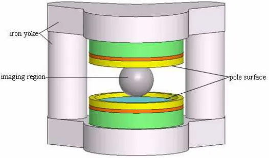
Figure 1. Structure of MRI magnet.

2. PROCESS OF PASSIVE SHIMMING

The principal structure of an open permanent main magnet for MRI is shown in Fig. 1. The imaging region is a spherical volume with its diameter of 400 mm. The inhomogeneity, η, of the magnetic field in the region is defined as

η = Bmax−Bmin

Bmean ×10

6 ₍₁₎

where the unit of η is usually expressed by ppm (part per million).

Bmax and Bmin are the maximum and minimum of the magnetic flux density in the region respectively, while Bmean is the average value of the magnetic flux density in the imaging region.

With the manual shimming, the position and number of compensating shims are tentatively determined by shimming engineer. However, the process is completed by at least two engineers spending 5∼6 days and using thousands of shims. Besides, there are many shims used, and their distribution is irregular shown in Fig. 2. The amount of work is heavy and low efficiency in the process of manual shimming, hence its improvement is of significance.

3. FORMULATION OF THE METHOD PROPOSED

There is no current supply in the imaging region, so that the scalar magnetic potentialφsatisfies the Laplace equation

Figure 2. Sketch map of passive shimming.

that is, φ is a harmonic function. According to the properties of the harmonic function, the maximum and minimum of the function are all located on the boundary of the region. Thus the practical target area on which the homogeneity of magnetic field has to be checked is reduced and restricted onto the boundary of the region, the surface of the sphere.

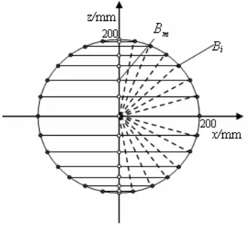
After the main magnet is assembled, the magnetic field on the spherical surface of the imaging region is measured firstly. The sampling values of the magnetic field are considered as “basic field”, which are measured using the magnetic field density meter PT2025, whose measurement range is from 0.043 T to 13.7 T, and its precision is 10−7T. The locations of the sampling points are shown in Fig. 3. The whole spherical surface is divided into 13 layers, and 12 sampling points located at equal interval are set on each layer, so that the data of 156 sampling points are gained. The passive shimming is programmed based on these data. In Fig. 3, which is the front view of the imaging sphere. Bmis the magnetic flux density on the longitudinal symmetrical axis and defined as the central magnetic field in the following text;Bi is the basic field value of theith point on the sphere surface.

Figure 3. Distribution of sampling points of the basic magnetic field.

upper hemispherical shimming is completed on the upper pole surface while the lower hemispherical shimming is completed on the lower pole surface. Shimming of the equatorial plane is finished on both of upper and lower poles.

According to Fig. 3, the values ofBmat the 13 points are measured from top to bottom. Generally, the homogeneity of these 13 points is very high, for example, the inhomogeneous value is only 7.699 ppm based on expression (1). If all the magnetic field of the points on the sphere is approached closely to the central value, the homogeneity of the imaging region will meet the imaging requirement. Therefore, the homogeneity of the central magnetic field provides a concrete reference for establishing shimming model. The process of shimming based on the central value is named as the central shimming strategy in this paper.

The central shimming method based on integer programming is proposed in this paper, which fulfills the combination of theory research and practical manual shimming. The objective function of peak-to-peak field tolerance subjected to series of inequalities is minimized, while the numbers and locations of small shims are regarded as objective variables. The possible positions of shims are previously set and their final positions are determined by the number of shims on corresponding position. When the shim number equals zero, no shim is set on the position. The mathematic model is given as expression (3) and (4).

st                    N X i=1

∆BijXi+Bj−Bm≤

T

2 for j = 1,2, . . . , M N

X

i=1

∆BijXi+Bj−Bm≥ −

T

2 for j= 1,2, . . . , M

−ni ≤Xi≤ni for i= 1,2, . . . , N

(4)

where λis a coefficient related to main magnet; T is the tolerance of the peak-to-peak magnetic field, whose expression isT =Bmax−Bmin;

Bmax and Bmin are the maximum and minimum of the magnetic flux density respectively;Xi(being integer) is the number of the superposed shims at location i;M and N are the total numbers of sampling and shimming points respectively;Bj is the magnetic field value measured at locationj on the spherical surface of the imaging region before the current shimming cycle, while Bm is the magnetic flux density at the center of measured plane; ∆Bij represents the change of the field at point j caused by a shim of a fixed size placed at locationi; and ni is the most number of shims at a shimming location.

4. SIMULATION TEST OF SHIMMING

The magnetic field created by a shim with a certain size and set on a certain position of a the pole surface is called as its “contribution” to the original basic magnetic field, which is equal to the difference of the magnetic field on the spherical surface before and after the placement of the shim. In order to avoid the difficulty of analytic solution, all the

The model described in Section 3 is solved using the branch and bound method [7–9] based on the software LINGO8.0. The initial data of magnetic field are measured in factory making magnets for MRI. After gaining each shimming scheme, a simulation test is implemented. The process of shimming simulation is divided into 3 steps. In order to examine the results of every shimming step, numerical analysis method is used to solve the whole contribution of the shim array.

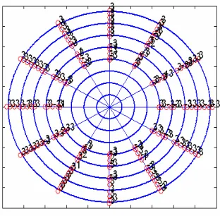
Step 1: Shimming along 12 lines with an interval of 30 degree on the pole surface (just shown as Fig. 5).

Figure 5. Schematic sketch of interpolation of the basic magnetic field with 15 interval.

Take the data of 156 sampling points firstly measured as the basic magnetic field. Build the integer linear programming model according to expression (3) and (4), and solve it to obtain the scheme of shimming based on the software LINGO Fig. 4 shows the computation results, which is used to direct the operator to do the shimming. Each small ring represents a position where shims locate, and the figure around it indicates the number of shims at the position in Fig. 4.

Step 2: Shimming along 12 lines with an interval of 30 degree and beginning from the 15 degree on the pole surface (see Fig. 5).

As shown in Fig. 5, the dashed lines demote the new shimming positions in this step. The new values of the basic magnetic field on the spheric surface are obtained by the interpolation between the values gained after Step 1. Then the integer programming model is solved to obtain the 15-degree shims distribution on the radial beam.

Based on the corrected data of Step 2, through interpolating, solving and shimming, the information of shims is obtained finally.

According to the final information of shims, which is obtained based on the above steps, the practical shimming is operated through sticking shims on both upper and lower poles. The shimming result is obtained through measuring the magnetic field on the imaging sphere surface with tesla meter.

In order to verify the availability of shimming algorithm in advance, the contribution of shim array is computed using numerical analysis. The difference between the magnetic field created by a small shim and the main magnet is great. The former is only 10−7T while the latter is 0.3 T. Considering the rounding error and truncation error of the finite element analysis, computation precision of the magnetic field value will not be accurate if the permanent main magnet and iron yoke are included in magnetic field analysis, so that the model of shim array is built with the imaging region set as solving area.

Figure 6 shows the physical model of shimming scheme built with the software ANSOFT [10].

Figure 6. Total information of shims array.

Figure 7. Distribution of the magnetic flux density and the inhomogeneity of the basic field (η= 1813.0111 ppm).

Figure 8. Distribution of the magnetic flux density and the inhomogeneity after shimming (η= 860.16 ppm).

Table 1. Comparison of the inhomogeneity before and after shimming (magnet 1).

Step Step 1 Step 2 Step 3

η0 (ppm) 1813.01 1144.00 928

Table 2. Comparison of the inhomogeneity before and after shimming (magnet 2).

Step Step 1 Step 2 Step 3

η0 (ppm) 1081.82 911.14 681.857

η1 (ppm) 911.14 681.857 637.46 ∆η/η0 (%) 15.78 25.16 6.5

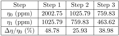
Table 3. Results of the shimming experiments. Step Step 1 Step 2 Step 3

η0 (ppm) 2002.75 1025.79 759.83

η1 (ppm) 1025.79 759.83 463.62 ∆η/η0 (%) 48.78 25.93 38.98

The above tables indicate that the total homogeneity of two main magnets after twice shimming is separately improved 52.56% and 41.08%. That is to say, the shimming schema of the central magnetic field is effective. The information of shims can be obtained easily. The homogeneity of different basic magnetic field can be improved in a wide range.

In order to check the precision of the shimming algorithm proposed in this paper, shimming experiment of the queen-post permanent magnet is completed in the enterprise that produces the magnet used for MRI. The results of shimming is shown in Table 3. Comparison is done to the same magnet between the manual shimming method and the central shimming method. The number of shims is 1400 for the central shimming while the manual is nearly 10000; The time of the central shimming is only 2 days, which includes time of computing just 3 minutes a time and setting the shims, while the manual shimming of one proficient engineer costs more than 5 days.

5. CONCLUSION

process. Corporation with the manufacturing enterprise shows that the method proposed is quite efficient. The profound research of the method proposed in this paper needs to be done to make the homogeneity meet the imaging requirements

ACKNOWLEDGMENT

Supported by the Doctoral Program Foundation of Institutions of Higher Education of China under Grant 20050142003.

REFERENCES

1. Wilkins, J. and S. Miller, “The use of adaptive algorithms for obtaining optimal electrical shimming in magnetic resonance imaging (MRI),”IEEE Trans. on Biomedical Engineering, Vol. 36, No. 2, 202–210, 1989.

2. Yamamoto, S., T. Yamada, M. Morita, et al., “Field correction of a high-homogeneous field superconducting magnet using a least squares method,”IEEE Trans. on Magnetics, Vol, 21, No. 2, 689– 701, 1985.

3. Belov, A. and V. Bushuev, “Passive shimming of the supercon-ducting magnet for MRI,”IEEE Trans. on Applied Superconduc-tivity, Vol. 5, No. 2, 679–681, 1995.

4. Lopez, H. S., F. Liu, E. Weber, et al., “Passive shim design and a shimming approach for biplanar permanent magnetic resonance imaging magnets,” IEEE Trans. on Magnetics, Vol. 44, No. 3, 394–402, 2008.

5. Dorri, B. and M. E. Vermilyea, “Passive shimming of mr magnets: Algorithm, hardware, and results,” IEEE Trans. on Applied Superconductivity, Vol. 3, No. 1, 254–257, 1993.

6. Wang, E., “The passive shimming technique research for a special application of the permanent magnet,” Shenyang University of Technology, Shenyang, China, 2007 (in Chinese).

7. Van de Panne, C. and F. Rahnamat, “The first algorithm for linear programming: An analysis of kantorovich’s method,”Ecnomics of Planning, Vol. 19, No. 2, 76–91, 1985.

9. Armstrong, R. D. and P. Sinha, “Improved penalty calculations for a mixed integer branch-and-bound algorithm,” Mathematical Programming, No. 6, 212–223, 1974.