Western University Western University
Scholarship@Western
Scholarship@Western
Electronic Thesis and Dissertation Repository
6-21-2017 12:00 AM
Essays on Entertainment Analytics
Essays on Entertainment Analytics
Kyle Maclean
The University of Western Ontario
Supervisor Fredrik Odegaard
The University of Western Ontario Graduate Program in Business
A thesis submitted in partial fulfillment of the requirements for the degree in Doctor of Philosophy
© Kyle Maclean 2017
Follow this and additional works at: https://ir.lib.uwo.ca/etd
Recommended Citation Recommended Citation
Maclean, Kyle, "Essays on Entertainment Analytics" (2017). Electronic Thesis and Dissertation Repository. 4683.
https://ir.lib.uwo.ca/etd/4683
This Dissertation/Thesis is brought to you for free and open access by Scholarship@Western. It has been accepted for inclusion in Electronic Thesis and Dissertation Repository by an authorized administrator of
This thesis explores live entertainment analytics and revenue management allocation strategies for live entertainment.
In Chapter two, we look at empirical factors that effect the success of Broadway shows. How well-known actors (stars) effect film revenues has been a recurring question of entertain-ment producers and academics. Because a film cannot be disentangled from a star involved, researchers have long struggled to rule out “reverse-causality” - that stars have access to higher quality movies. Using a novel data set that includes Broadway show revenues and actor usage, we provide a fixed-effects regression and case studies. We find across multiple specifications that increases in star power in a show improve revenue.
Motivated by social grouping and the associated operational challenges, in Chapter three we formulate and study extensions to the Dynamic Stochastic Knapsack Problem (DSKP). We compartmentalize the knapsack according to predefined reward-to-weight ratios, and in-corporate a stochastic interaction between the offered set of open compartments and the item placement. Using a specific interaction function inspired by customer choice in the entertain-ment industry, we provide an algorithm to determine the optimal solution and obtain insights into structural properties. Given the computational complexity of the dynamic program we also propose and analyze via simulation a heuristic algorithm.
In Chapter four, in a large sequence of simulations, we propose and study practical heuristic algorithms on which seats should be offered to requests. We propose an algorithm that offers revenue improvements from a “naive” policy on the order of 5-10%.
Throughout, we aim for managerial relevance, providing implications to current techniques both in strategy as well as operations.
Keywords: Entertainment, Revenue Management, Markov Decision Process, Simulation, Seating, Operations
Co-Authorship Statement
I declare that this thesis incorporates some material that is a result of joint research. Chapter three “Dynamic Stochastic Knapsack Problem with Adaptive Interaction:Live Entertainment Capacity Based Revenue Management” and Chapter four “A Simulation Analysis of Group Seating Heuristics” are co-authored with Dr. Fredrik Odegaard. As the first author, I was in charge of all aspects of these projects including formulating research questions, literature re-view, model formulation, simulation programming, and preparing the first and the following complete drafts of the manuscript. With the above exceptions, I certify that this dissertation and the research to which it refers, is fully a product of my own work. Overall, this dissertation includes 3 original papers.
Abstract ii
Co-Authorship Statement iii
List of Figures vi
List of Tables vii
List of Appendices viii
1 Introduction 1
2 Mega-Stars and the Blockbuster Strategy: An Empirical Analysis of Broadway
Revenue 5
2.1 Introduction . . . 6
2.2 Background and Literature Review . . . 7
2.2.1 Literature Review . . . 7
2.2.2 Endogeneity in Actor Selection . . . 7
2.2.3 Broadway Background . . . 9
2.3 Model Framework . . . 10
2.3.1 Broadway Data . . . 12
2.3.2 Dependent Variable: Weekly Gross Revenue . . . 13
2.3.3 Independent Variables: Operationalization of Star Power . . . 14
2.4 Results . . . 18
2.4.1 Graphical Analysis . . . 18
2.4.2 Regression Results . . . 23
2.4.3 Model Results . . . 23
2.4.4 Model Diagnostics . . . 25
2.4.5 Case Studies . . . 26
American Idiot . . . 26
How to Succeed in Business Without Really Trying . . . 29
2.5 Discussion and Conclusion . . . 30
3 Dynamic Stochastic Knapsack Problem with Adaptive Interaction: Live Entertainment Capacity Based Revenue Management 33 3.1 Introduction . . . 34
3.1.1 Literature Review . . . 36
3.1.2 Technical and Managerial Contributions . . . 37
3.2 Knapsack Model Formulation . . . 38
3.2.1 Optimality Equations . . . 39
3.2.2 Monotonicity Properties . . . 42
3.3 Entertainment Knapsack Problem . . . 44
3.3.1 Transactional Data-Driven Estimation of Row Selection . . . 44
3.3.2 Customer Choice Model Based Row Selection . . . 45
Threshold Based Policies . . . 48
3.3.3 Numerical Illustration . . . 51
3.4 Single-Row DSKP Heuristic . . . 53
3.4.1 Single-DSKP Heuristic Algorithm . . . 53
3.4.2 Simulation Study . . . 54
3.5 Conclusion . . . 55
4 A Simulation Analysis of Group Seating Heuristics 57 4.1 Introduction . . . 58
4.2 Literature Review . . . 58
4.3 Venue Seat-Selection Process . . . 59
4.4 Seat Offering Heuristics . . . 62
4.5 Simulation Study . . . 66
4.5.1 Simulation Parameters . . . 66
4.5.2 Simulation Results . . . 66
4.6 Discussion and Conclusion . . . 70
5 Conclusion 72
Bibliography 75
A Other Data and Models 79
B Proofs of Theorems 82
Curriculum Vitae 89
1.1 Weekly potential gross for selected shows in 2016. . . 3
2.1 Conceptual Model for Films . . . 11
2.2 Conceptual Model for Broadway . . . 11
2.3 Screenshot of example raw role information from IBDB.com . . . 13
2.4 Boxplots of selected shows’ weekly grosses . . . 14
2.5 Screenshot of the STARmeter graph from IMDB.com . . . 15
2.6 Histogram of non-zero STARmeter values in our dataset on 6/30/2015. Each bin width is 0.05. . . 16
2.7 Scatterplots of independent variables Starpower and Starpower3 against depen-dent variable Gross . . . 21
2.9 Residual diagnostics for four models . . . 27
2.10 American Idiot performance relative to control group . . . 28
2.11 How to Succeed performance relative to control group . . . 30
3.1 Screenshot of the Broadway Musical Aladdin’s seating chart. Source: Ticket-master.com . . . 35
3.2 Decision Tree of Numerical Example . . . 41
3.3 CDF of wtp and resulting row preferences. . . 47
3.4 results from Numerical Illustration. . . 52
3.5 Summary of Simulation Study. . . 54
4.1 A 20 row, 30 column venue with heat map ofur,c values whenβ = 1. Front of the stage is the bottom of the figure. s1,15is the best seat in the venue. . . 61
4.2 A 20 row, 30 column venue after 100 arrivals of group typei= 1, with differing βparameter . . . 62
4.3 Sequence of Events . . . 63
4.4 A comparison of offered sets for three heuristics at a 20 row, 30 column venue with ani= 3 group arriving . . . 67
4.5 Box plots of percent difference between given algorithm and NAIVE in a given trial under theα1 = 5% condition . . . 68
4.6 Box plots of percent difference between given algorithm and NAIVE in a given trial under theα1 = 10% condition . . . 69
List of Tables
2.1 Example Actors for adjSTARmeter values . . . 16
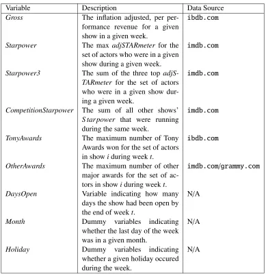
2.2 Variable Descriptions . . . 19
2.3 Correlation Matrix . . . 19
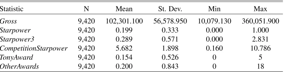
2.4 Summary Statistics of Variables . . . 20
2.5 Mean Values for Star Weeks compared to Non Star Weeks . . . 20
2.6 Regression Results . . . 24
2.7 Estimated effects from hiring single actor with adjSTARMeter=0.98 . . . 25
2.8 Estimated effects from hiring two actors with adjSTARMeter=0.7 each . . . 25
2.9 Summary Statistics of American Idiot Grosses. Star Weeks are defined as those which included Billie Joe Armstrong. . . 26
3.1 Table of Numerical Illustration parameters. . . 51
4.1 Group Distribution Configurations . . . 67
A.1 List of Holidays Controlled for in Chapter Two . . . 79
A.2 Regression Results from all models in Chapter Two . . . 80
A.3 Regression Results from Chapter Two assuming random effects on unobserved individual characteristics. . . 80
Appendix A Other Data and Models . . . 79 Appendix B Proofs of Theorems . . . 82
Chapter 1
Introduction
The entertainment business is fascinating, containing many unique strands that differentiate it from other industries. In this thesis, we explore these different facets analytically and discuss how managers can face them. In general, we explore two different ideas: the uncertainty of success, and operational allocation of seats.
In virtually all entertainment fields (e.g, films, live theatre, books...etc), there exists a winner-take-all element. Successful entertainment products do tremendously well and cap-ture a large share of revenues, while the majority of products make meager revenues. The problem managers face is that the process of becoming a winner is highly uncertain, and path-dependent (Salganik et al., 2006). William Goldman, a Hollywood screenwriter, once said that “nobody knows anything” about what makes a movie successful (Goldman, 1983).
The entertainment industry is interesting from an operational point of view as well. The in-dustry generally satisfies the criteria of Revenue Management (RM) methodologies; There is a fixed-supply of seats that become perishable after an event, and selling an extra seat incurs low marginal costs. However, live entertainment is different from traditional RM application areas such as airlines. As mentioned above, social factors are more important, and the experience is more uncertain prior to purchase.
The key interlinking idea between these two topics is exploring how businesses should make decisions in an environment where social factors are important and groups of consumers make and engage in purchasing decisions. This creates research questions on an operational level (How to offer seats to incoming groups?) as well as at a strategic level (Should films and live entertainment products focus on “stars”?).
The predominant focus within the RM literature on live entertainment has been regarding pricing (or value) and its effect on demand/sales. For instance, Leslie (2004) examine Broad-way data and show that seat price discrimination improved profit by 5% relative to uniform pricing; Hume et al. (2006) examine factors influencing service quality in performing arts; Toma and Meads (2007) empirically explore macro-level determinants of symphony atten-dance; Veeraraghavan and Vaidyanathan (2012) developed and empirically analyzed location based “seat value” and customer utility of events (specifically baseball); and Dixon and Verma (2013) show how sequence effects play a significant role in influencing season subscription renewals.
A main focus of RM in general is on differential pricing. This comes in the form of dy-namic pricing andvariable pricing. In the live entertainment sphere, dynamic pricing refers to changes in prices over time based on changes in realized demand vs predicted demand. For management simplicity, dynamic pricing often uses capacity levels as triggers to alter pricing. For example, to raise prices when 10% of capacity remains.
Variable pricing refers to different prices for different products, where a product is a spe-cific seat to a spespe-cific event. Variable pricing is common in live entertainment. For example, a Friday night show may be priced differently than a mid week matinee. The event itself some-times differs materially too. Sports teams sometimes change prices depending upon who is being played.
3
$1,000,000 $1,500,000 $2,000,000 $2,500,000
Jan 16 Apr 16 Jul 16 Oct 16 Jan 17
W
eekly P
otential Gross
Aladdin The Book Of Mormon The Lion King Wicked
Figure 1.1: Weekly potential gross for selected shows in 2016.
the house”.
Dynamic pricing in live entertainment has only begun to be introduced recently but has spread to multiple outlets. Major League Baseball’s (MLB) San Francisco Giants introduced dynamic pricing to the sports industry in 2009 (Kemper and Breuer, 2016). In 2012 , 17 MLB organizations were beginning to dynamically price their events in some fashion Dunne (2012). On Broadway, sophisticated RM pricing methods are often associated with Disney produc-tions, sometimes cited as the “masters” of the process (Healy, 2014). In some of its shows, management sets limits on how high prices can be set, ostensibly to keep prices affordable for families. Other shows on Broadway are generally independently organized and financed, making sophisticated RM processes more unlikely.
To test the extent of these RM techniques on Broadway, we use publicly available data about shows’ weeklypotential gross. Potential gross measures how much a production could possibly make in a given week. The calculation is the summation of each seat, at each perfor-mance, at the posted price for that week. I.e. coupons and other discounts are ignored, and so a show can be fully attended without reaching 100% of its potential gross. We hypothesize that an active RM pricing regime would result in changes in prices week to week and thus differing potential gross numbers.
In Figure 1.1 we plot potential grosses for four selected shows on Broadway in 2016. Note the two Disney productions (Aladdin and The Lion King) exhibit changes week to week and throughout the entire year. In fact, it is rare to see two weeks where potential gross does not change. This is consistent with an active variable pricing process. In contrast, we look to Wicked and Book of Mormon, two other successful shows on Broadway. These two shows exhibit very long periods of unchanged prices, even during strong seasonal trends, e.g. the summer tourist season. However, even these shows exhibit temporary bumps during holiday periods - note that all shows have relatively higher potential grosses at the start of January 2016 - the week including the previous New Year’s Eve.
that stars/budgets/marketing are a successful strategy in entertainment. However, because a film cannot be disentangled from a star involved, researchers have long struggled to rule out “reverse-causality” - that stars have access to higher quality movies. We argue that the com-mercial live-theatre environment provides a way of controlling for a show’s fixed effects. Using a novel data set that includes Broadway show revenues and actor usage, we provide a fixed-effects regression and case studies. We find across multiple specifications that increases in star power in a show improves revenue. We also find that competitive star power has a negative, but not statistically significant effect on revenues. We discuss managerial implications as well as directions for future research based on the Broadway context.
Motivated by social grouping and the associated operational challenges, in Chapter two we formulate and study extensions to the Dynamic Stochastic Knapsack Problem (DSKP). We compartmentalize the knapsack according to predefined reward-to-weight ratios, and in-corporate a stochastic interaction between the offered set of open compartments and the item placement. Using a specific interaction function inspired by customer choice in the entertain-ment industry, we provide an algorithm to determine the optimal solution and obtain insights into structural properties. Given the computational complexity of the dynamic program we also propose and analyze via simulation a heuristic algorithm.
In Chapter three, for tractability, we assume that groups are seated strictly from left to right, arguing that this can be operationalized by managers. In Chapter four, we relax this assumption and allow incoming requests to sit anywhere within a row. In a large sequence of simulations, we propose and study practical heuristic algorithms on which seats should be offered to requests. We find that a “naive” offer-all method is inefficient across a wide variety of conditions. We propose an algorithm that offers revenue improvements on the order of 5-10%, and show how it compares to common industry methods.
Chapter 2
Mega-Stars and the Blockbuster Strategy:
An Empirical Analysis of Broadway
Revenue
2.1
Introduction
Entertainment industries (e.g films, live theatre, books, etc.) face a winner-take-all environ-ment. The “winners” grab the vast majority of the revenue while losers make relatively little (Vany and Walls, 1999). Cultural products like films and theatrical productions face high up-front costs with highly uncertain lifetime revenues. The Blair Witch Project, with a budget of $60,0001eventually made over $200MM at the box office. At the same time, the 2016 summer
filmBen-Hurcost $100MM to produce, and only made $94MM in domestic revenue.
A constant managerial question is what actions can be taken to increase the probability of success, or mitigate the probability of failure. The screenwriter William Goldman once said that in the movie industry “Nobody knows anything”. Similarly, Jeffrey Sellers, the producer behind the mega-hit Broadway musical Hamilton suggested that “there is no moneymaking formula on Broadway” (Sokolove, 2016).
One formula suggested has been the “blockbuster” strategy. A “blockbuster” strategy en-tails using high production values, copious amounts of marketing, and well known actors (stars) to try to create extreme winners (Elberse, 2013). In the movie business, this can imply using known intellectual property (sequels), stars, and high marketing budgets to produce “tent-pole” summer productions. However, academic evidence for this strategy is mixed and popular reac-tion to it has varied. The media has suggested that the strategy has died off. A 2016 summer NY Times article was titled “ Hollywoods Summer of Extremes: Megahits, Superflops and Little Else”. A Vox article was titled “Hollywoods go-to formulas [have] stopped working”.
One aspect of the blockbuster strategy is using stars to create a hit. Using stars can spur an information cascade, causing herd behavior in consumers (Bikhchandani et al., 1992). Stars also have a high cost though, both financially and logistically. Determining how and whether stars affect financial success is the first step to answering whether these costs are worthwhile. The literature to date on this question has been mixed, and definitive answers are unclear. Some papers find that stars increase film revenue. Others find that no effect or only an indirect effect. Much of this uncertainty in the literature stems from the inability to clearly identify causality. In a film, a star may be correlated with other movie characteristics, such as quality stories, scripts, budgets, and other creative elements. This has been referred to as the “reverse-causality” problem (Liu et al., 2014).
To address this issue, we propose looking at the live theatre environment, where different actors perform in the same show over time. We obtain a novel data set of which actors were present in Broadway productions in a given week, and weekly grosses of those shows. Using a continuous measure of star power, we study how a show’s star power drives weekly revenue. We find that increases in star power improve revenues on average, as do major awards, except for Tony awards. Our work builds on a recent effort to correct for endogenous actor selection (Liu et al., 2014) and finds that stars directly, rather than indirectly effect revenues. We also explore competitive effects, finding a negative but not statistically significant effect of other Broadway shows hiring stars. We discuss managerial implications as well as future research directions.
2.2. Background andLiteratureReview 7
2.2
Background and Literature Review
2.2.1
Literature Review
A variety of mechanisms and conceptual models have been proposed for how stars might alter the success of entertainment products. Most literature here is centered in the film industry con-text. Albert (1998) proposed that stars serve as a “marker” of a successful film type. Similarly, Thomson (2006) and Luo et al. (2010) suggested that stars are a type of human brand. A star might signal the type or quality of a cultural product that a consumer might purchase. For example, a consumer may update their private beliefs about the genre/quality of the movie if the consumer realizes a certain star is involved. In that way, a star would reduce the quality risk for consumers. Cultural products, being experiential goods, have quality that is difficult to predict a priori. It would hold then, that if consumers have a better idea of the type of film, demand may increase.
A rich literature has been developed to empirically test this theory in business environments, with almost all of the literature being based in the film industry. Unfortunately, empirically the literature is mixed. Some find a positive effect from using stars. Using an online prediction market as an event study, Elberse (2007) finds that stars have a statistically significant posi-tive relationship with revenues, and is able to determine the value of specific actors. Nelson and Glotfelty (2012) use IMDB rankings to operationalize star power, and apply a per-country regression, finding a statistically significant positive effect of stardom. Other papers find no statistically significant effect.Prag and Casavant (1994) find no significant effect, after account-ing for marketaccount-ing expenditures, from a star’s presence in a movie. But the authors note that the presence of a star also effects marketing expenditures. Ravid (1999) comes to a similar conclusion, noting that when including budgets, stars do not seem to significantly effect rev-enues. Vany and Walls (1999) use a distributional approach and conclude that stars do not make successful films, the movie itself does. In a fascinating new work, Liu et al. (2014) create an endogenous switching model to control for endogenous matching processes. They find that any effect stars have on revenues is largely indirect, from different movie characteristics as well as increased theatre allocation (i.e. stars cause their movies to be in more screens nationwide).
Other work has researched other factors that stars may effect. Joshi (2015) focused on week-to-week grosses, rather than total grosses, and found that they had less volatility when a film had a star. If the movie business values consistent cash flow, week-to-week riskiness should also be important to them. Liu et al. (2013) finds that stars impact stakeholders in the early project stages (e.g. financing and pre-production) but that the impact on audience may again only be indirect.
When positive results are found, most of the literature has only claimed that their result is an association, rather than causation. This is due to endogeneity in the process of matching star actors with films.
2.2.2
Endogeneity in Actor Selection
through a complex sequence of bargaining and access (Ravid, 1999). This implies that actor selection is endogenous and potentially related to movie characteristics (Liu et al., 2014).
Endogeneity between star power and movie characteristics is bi-directional. Star actors, if they have bargaining power, may be able to influence or seek out specific film characteristics of projects that they are involved in. Given private information about characteristics that go into the quality of a product, star talent may choose projects that are projected to have higher quality. Alternatively, from the producer side, producers may choose to attach stars to specific movies (Eliashberg et al., 2006). They may do so to ensure project financing. Furthermore, they may attach stars only to specific genres.
If these forms of endogeneity exists, it presents a problem for empirically assessing the inclusion of a star in a cultural product. Stars may beassociatedwith higher revenues, but only through their association with other movie characteristics. As Vany and Walls (1999) points out, the movie would make the star, instead of the reverse. “Reverse - causality” would remain a potential explanation.
Endogeneity could be dealt with partially through more data. Some movie characteristics are possible to control for by obtaining more data. For example, much of the literature includes budget as an independent variable in the analysis. However, others would be very difficult, if not impossible to quantify and operationalize (e.g the quality of script/story)
Numerous papers have identified this issue as well. Eliashberg et al. (2006) states the need for continuing research into what effect stars have on films. Elberse (2007) points out the reverse-causality issue and attempts to solve it via the event study approach on a public pre-diction market. Given full information, a prepre-diction market would identify the effect a change in actor has on estimated revenues. Thus, an event study would solve this issue. However, as Ravid (1999) points out, and Elberse (2007) acknowledges, there is assymetric information in the market for films and full information is not available to the prediction market. Script qual-ity, budget, and other movie characteristics may be unknown to the prediction market. With assymetric information, the presence of a star can serve as a signal of these other movie char-acteristics. Thus, even under the null hypothesis of no effect, the prediction might change as a result of the announcement in stars. Therefore, if the prediction market operates on public in-formation, which the online website does, an event study using prediction markets still suffers from the same issue of a reverse-causality explanation.
Liu et al. (2014) formalizes the notion of endogeneity in the film market and star selection. They attempt to solve the issue via explicitly modelling actor selection and movie characteris-tics. However, the study only seeks to measure opening week differences. Our study is cleaner in the sense that star power variation occurs naturally over time on Broadway. Furthermore, we notably find different results. Liu et al. (2014) find that stars increase the number of screens a film is on. On Broadway, capacity changes are not possible since a theatre’s number of seats is fixed. Thus, we find a different mechanism than them.
2.2. Background andLiteratureReview 9
prior to the show starting2, the actual performance occurs nightly before a live audience.
2.2.3
Broadway Background
Broadway theatres refers to 41 professional theatres in downtown New York City. A Broad-way theatre is classified as any downtown theatre with more than 500 seats. Capacity varies widely though; the smallest theatre has 597 seats, while the largest has 1,935 seats. Shows on Broadway are generally categorized as either plays or musicals.3 Plays are scripted
produc-tions, while musicals incorporate songs with singing and choreography, in an often extravagant manner.
Shows can be categorized as being open ended runs or limited runs. A “run” refers to the amount of time that a show will be playing for. Open ended productions have no specified end date and will run for as long as the show is profitable. A limited run is a show that opens and has a specified end date. Limited runs are common with plays that open with star actors, because of their busy schedule (Reaney, 2014). However, even limited runs can extend their run given heavy demand, depending on the schedule of their cast and on the availability of their theatre. The standard running week of a Broadway show is 8 performances every 7 days, with one “dark” day where no performances are held.
A Broadway project generally progresses according to the following sequence. The show undergoes rehearsal for 2-4 weeks where the cast and creative team rehearse and practice the show. During the final week, a “tech” rehearsal occurs where the lighting and sound elements are brought together with the cast and cues synced. Once public performances begin, a show goes through several weeks of previews. During previews, the general public buys tickets to the show understanding that design elements may change or be a work in progress. Musicals for instance may remove songs, edit dialogue, and alter staging during the preview period. On opening night, the show is locked and no further creative elements are changed4. In addition,
professional reviewers (e.g. The New York Times, The Washington Post) publish their official review of the show on opening night.
Commercial theatrical productions on Broadway can be long running affairs: The Lion King on Broadway has been running for over 18 years with over 7500 performances. In long running shows, while the creative elements are fixed, the actors themselves change throughout the run of the show. Like in the film industry, actors are chosen based on a negotiated match-making process. This would involve both their acting ability as well as their potential star power to draw in an audience. Star actors sometimes headline the show during the beginning of a run in hopes to generate interest. This occured in 2011 when the revival ofHow to Succeed
in Business Without Really Trying opened. Daniel Radcliffe, from Harry Potter fame, was
cast as the lead character and played the role for a little less than a year (Feb 26, 2011 - Jan 01, 2012). Stars however can also be replacements during the middle of the run, sometimes negatively referred to as“stunt-casting”, because of the perceived lack of talent of these actors.5
2Minor changes to scripts can occur during previews, or sometimes during extended runs however.
3Exceptions exist: The magic show Penn & Teller is not obviously described by these labels.
4Some small topical references that become outdated can be edited, e.g. after the presidential election in 2008,
the musical Avenue Q altered a lyric referencing George W Bush.
In the musicalIn the Heights, High School Musical star Corbon Bleu stepped into the lead role partway through its run (Jan 25, 2010 - Aug 17, 2010).
The years in our dataset were years of change on Broadway. Revenue management (RM) techniques like variable pricing became more common, spearheaded by Disney and its produc-tions (e.g. The Lion King) (Healy, 2014). From 2009 to 2015 the average price for sold tickets increased from $83.02 to $104.26, a 25% increase that far outpaced inflation. Prices changes like this could be a result of more pervasive RM techniques, or as a result of shifting consumer preferences toward live entertainment.
While the industry has changed, in this chapter we focus solely on the effect of starpower, not necessarily the prediction of grosses in general. Changes in pricing behavior with respect to RM behavior should not create bias in our estimated effects of starpower.
Our research thus also intersects with a literature on the success of live theatre. This litera-ture generally centers around what effects the success of a show, as well as how awards or re-views can effect a shows revenue. Reddy et al. (1998) examine multiple factors that impact the success of a Broadway show including critic reviews and advertising expenditures. They find that critics both predict and influence success. The authors also investigate the effect of actor choices, using as proxies the total number of shows on Broadway the lead cast/director/author had done, as well as the number of awards these individuals received. Boyle and Chiou (2009) examine the value of winning a Tony Award using a discrete choice model as well as a hazard model. They suggest that nominations bring general positive increases to all shows, but that attention shifts to just the winners after the awards are given. They also propose that awards information follows as an information cascade where the main effect is not felt immediately. Simonoffand Ma (2000), using a survival model found mixed results for major paper reviews, but a positive effect from winning awards. Maddison (2004) also performed a survival analy-sis on Broaday shows, finding that original shows tended to outlast revivals. The author also finds that as shows last longer, the more likely they are to last for a longer time, unlike in the movie industry. Maddison (2005) looked into revivals on Broadway, finding that revivals are becoming more prevalent and that they are less risky, though do less well on average.
Notably, Reddy et al. (1998) investigates how actors affect lifetime revenue on Broadway, however only do so based on the actors who were there on opening night. This is an interesting question but suffers from the same direction of effect questions as the film industry. This analysis was only done for the opening night cast and did not test what happened when these lead actors left the show and thus, similar to the movie industry, this approach is not able to cleanly identify star power effects.
2.3
Model Framework
2.3. ModelFramework 11
Figure 2.1: Conceptual Model for Films
Weekly Revenue Cast
Pre-Production
Film Quality Capacity (Number of Screens) Other Creative Elements
(Script/Director/Genre/Budget)
Seasonality/Holidays
Figure 2.2: Conceptual Model for Broadway
Weekly Revenue Cast
Pre-Production
Show Quality Capacity (Number
of Screens)
Other Creative Elements (Script/Director/Genre/Budget)
Seasonality/Holidays
very inflexible. Although it is possible for a show to switch theatres during its run, the switch is very expensive, lengthy, and ultimately rare. Capacity is therefore non-dynamic throughout a show’s run.
Quality levels can differ on Broadway throughout a show’s run, in contrast to film. By qual-ity, we mean the general artistic ability to provide intended emotions to an audience. Changes in actors may effect the quality of a show through changes in innate acting ability or ability to perform in a live show. For example, it was reported that Bruce Willis in 2015 had to be fed lines through an earpiece on stage6.
We do not explicitly include changes in quality in our model, largely because data is not available. However, we argue this effect is small. Producers have a vested interest in keeping the quality of their own show at some minimum level. In addition, if quality had high temporal variability we would expect to see new reviews of shows on cast changes. This is rare, indicat-ing that quality, although theoretically effected by cast, is for practical purposes steady. Thus, although in theory quality may be variable over time, in our model quality is captured by the time invariant unobserved effects of a show.
In our model, we index shows by i = 1, . . . ,N; where N is the number of shows in our sample. We index time (weeks) byt= 1, . . . ,T, wheret=1 is the first week in our sample (the week ending May 31st 2009) andt= T is the last week in our sample (the week ending August 1st 2015).Our dependent variable is the log transformed weekly per-performance revenue,yit
for showiin weekt. xitis a column vector ofKexplanatory variables for showiin weekt.
More details are provided about the specific independent variables in xit in Section 2.3.3.
Details about the dependent variable yitare given in Section 2.3.2. Variables are summarized
in Table 2.2. Our econometric model is given by
yit =βx0it+αi+it
fori=1. . .N,
fort=Tsi. . .Tei,
where Tsi is the starting week for show i and T i
e is the ending week. β is the column vector
of parameters/coefficients. αi is the unobserved individual effect of show i, that is intended
to capture time-invariant heterogeneity. it is the idiosyncratic error term which is assumed to
be independently distributed across shows but with a potential dependence across time (We assume thati ∼ i.d.(0,Ωi)). That is, we explicitly allow for within showiserial correlation in
errors and heteroskedasticity.
We assume that αi is a fixed effect, rather than a random effect. A random effects would
require the assumption thatαi is uncorrelated with the entries of xit. In our context, this
as-sumption would imply that star power is uncorrelated with script/budget/genre. This is a strong assumption and one we do not wish to make. Therefore in our analysis we assume thatαi are
fixed effects7. Each αi is treated as an unknown parameter to be estimated (Greene, 2007, p.
359).
The theoretical downside to modeling αi as a fixed effect is that time-invariant covariates
would not be able to estimated, since they would be captured by αi. For our purposes, this is
acceptable since we are not interested in time-invariant factors (e.g. genre, budget) and explic-itly do not include them in our model. We are specifically focused on variation in starpower over time. However, this does mean that shows who had no replacement in actors are not able to contribute to our estimation of starpower effect.
β and αi can be estimated using Ordinary Least Squares (OLS). However, since OLS
as-sumesit are i.i.d., the associated standard errors onβ andαi are generally biased downward
(Cameron and Miller, 2015, pg. 3). We instead use robust standard errors following Cameron et al. (2011) to account for any potential serial correlation or heteroskedasticity. This two-step procedure (OLS and robust standard errors) is mentioned by Cameron and Miller (2015) as a more recent method in the literature.
2.3.1
Broadway Data
We collected data from the Internet Broadway DatabaseIBDB.com, a website ran by the trade association for the industry, for all shows that were running during the period May 31st 2009-August 1st 2015. This resulted in 290 shows across 327 weeks . The 2009 starting date was chosen due to a change in reporting standards in grosses prior to that date. This data included the “gross gross”8 of each broadway show, in each week that it was playing. Revenue data is publically available and generally released every Monday, giving grosses for the previous week.
From the same site, we obtained information on which actors played which characters for all shows within the sample period. We refer to character/actor combination as “Roles”. Role information included the actors names, the character(s) they played in the show, and the dates they joined and left the show. Figure 2.3 shows an example of the data on the site itself.Since a role is both a character and actor combination, some actors are included in the dataset in multiple roles over different time periods. We index roles byr =1, . . . ,R.
We made significant efforts to ensure the data was cleansed and precise. Role information were removed due to a lack of either a start date, ending date, or imprecise start/ending dates.
7A model assuming random effects is presented in the Appendix however for robustness. All qualitative results
presented here hold.
2.3. ModelFramework 13
Figure 2.3: Screenshot of example raw role information from IBDB.com
9 Generally speaking, roles that were removed were either less important characters (so-called
“ensemble” members) or non-notable actors. We also ensured that no roles conflicted with each other, e.g. data that specified two actors playing the same character in the same week. For those weeks that showed two actors overlapping the same part, we assumed that the actor with the shorter overall time period was actually in the show. This tended to occur for short vacation periods of the main actor.
After this data cleansing process, we had 928 unique roles in our data set. This consisted of 633 unique actors across 80 shows. The number of shows with role information is less than our entire show sample. This is primarily due to short show runs for which no actors changed and therefore for which IBDB did not provide starting/ending dates. The mean length of a show for which we have actor information was 133 weeks compared to 51 weeks across the entire show sample. In a fixed effects analysis, a show with unchanging actors does not provide information about the effect of those actors. Therefore not having information on these shows did not effect our analysis. On average, an actor in our dataset was in a show for 31.9 weeks before leaving the show.
2.3.2
Dependent Variable: Weekly Gross Revenue
The dependent variableyitis a log transformed per-performance revenue for each show for each
week in our sample10. Weekly grosses were inflation adjusted to 2015 values using monthly CPI data in the United States11, and subsequently adjusted to a “Per-Performance” measure
by dividing by the number of performances done in a specific week. This change was done to control for any non-standard number of performances held. In a typical week, a Broadway pro-duction runs 8 shows per week. However this can vary in previews (prior to a show opening), or because of special holidays throughout the year. For example, during the holiday season in December, it is not uncommon for some shows to have 10 performances on a given week. We refer to this variable as Gross. In Figure 2.4, we provide box plots ofGrossfor a sample of shows from our data set. We see that meanGrosscan vary considerably across shows. We
9For example, some data points only indicated a general month of when an actor started with a show.
10Monetary variables are particularly suited to being specified in logarithmic form (Wooldridge, 2012, pg. 193).
Figure 2.4: Boxplots of selected shows’ weekly grosses for 2009-2015. The mean weekly gross for the entire sample is $102,301.
$50,000 $100,000 $150,000 $200,000 $250,000
Aladdin American
Idiot
August: Osage County
Billy Elliot:
The Musical
How to Succeed
in Business
Without Really Trying
Mothers and Sons
Promises, Promises
The Book of Mormon
Gross
consider this indicative of different fixed effects. This could be capacity, i.e different theatre sizes or different show quality levels. We also see significant variation within each show. We postulate that at least some of this variation is due to changes in actors and starpower.
Our final data set of revenues is an unbalanced panel structure. The panel is unbalanced because of the opening and closing process of the shows, and so some shows do not have data for certain weeks.
2.3.3
Independent Variables: Operationalization of Star Power
To determine how within-show variation in star power explains changes in revenues, we must operationalize the concept of star power. One common approach in the literature is to assign a dummy variable indicating whether an actor was a star. We opted against this approach because we feel it misses the granularity that still exists between actors (Nelson and Glotfelty, 2012). Two stars that might both be classified as a star, might still have different levels of star power. That is, star power is best represented by a continuous variable, rather than a binary one. This is recognized in the media as well, who popularly refer to certain actors as “A-List” stars or “D-List” stars. Dummy variables also have practical operationalization issues. A researcher must still find some underlying variable to operationalize awareness and choose an arbitrary cutoffpoint. Otherwise, they subjectively assign the dummy variables values such as in Prag and Casavant (1994).
2.3. ModelFramework 15
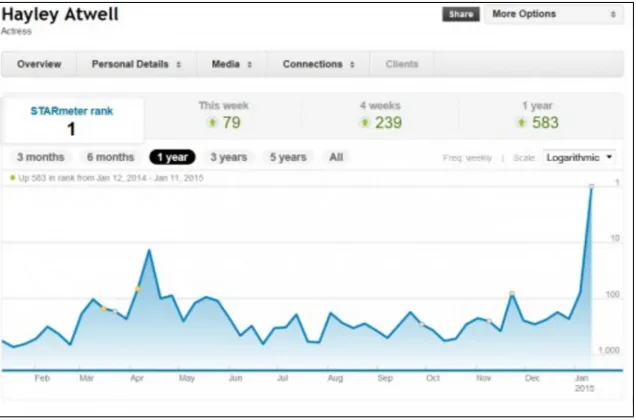
Figure 2.5: Screenshot of the STARmeter graph from IMDB.com
an advantage that such information is publically available and generally easily obtainable. We feel this is inappropriate for Broadway. Particularly recently, Broadway star actors have come from many industries. They may be successful movie actors (Daniel Radcliffe, Neil Patrick Harris), well known singers (Billie Joe Armstrong, Nick Jonas), television series actors (Matthew Morrison, Sean Hayes), or even well-known actors from Broadway (Kristen Chenoweth, Sutton Foster). Using film box office revenue does not allow us to measure star power across entertainment industries.
Instead we use the recommendation of Nelson and Glotfelty (2012) and use the IMDB STARmeter metric to quantify the popularity and star power of actors.12 This proprietary
ranking system uses search results on the IMDB platform to determine an up-to-date index of which actors are being viewed by the general public. On the website, STARmeter is a rank, such that the top actor has a ranking of 1, and increases in the ranking imply decreases in star power. Figure 2.5 gives an example of how STARmeter appears on the website, and how changes are graphed over time.
For each role, we collected the STARmeter rank of the actor on the date they joined the show13. A linear interpolation was performed for start dates that were between STARmeter
dates available.
To aid in interpretation, we made two adjustments to the raw data. We assumed that the difference in starpower between low-ranked actors was negligible and truncated it to 20,000. That is, for each STARmeter found, we took the minimum of it and 20,000. 20,000 was chosen because actors beyond this point are not recognizable to us.
After truncating values, we transformed the raw STARmeter ranking into a metric be-tween zero and one, with increases in value implying more star power. We call this variable
12Conceptually, it may be important to recognize that the ranking does not measure sentiment. A frequently
searched actor may not be generally liked. We do not seek to measure this difference in our study.
13In approximately 11% of the roles, we were unable to find a corresponding IMDB profile. We assumed these
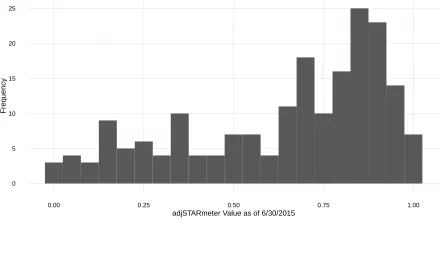
Figure 2.6: Histogram of non-zero STARmeter values in our dataset on 6/30/2015. Each bin width is 0.05.
0 5 10 15 20 25
0.00 0.25 0.50 0.75 1.00
adjSTARmeter Value as of 6/30/2015
Frequency
ad jS T ARMeter. We did this by applying the following formula, for roler,
ad jS T ARmeterr= 1−
min(S T ARmeterr,20000)−1
19999 . (2.1)
Thus, for the highest ranked star in a given week,ad jS T ARmeterrreturns one.adjSTARmeter
returns 0 if STARmeter is 20,000 with linear interpolation otherwise and with increases in value implying higher star power.
To provide context and better understand the range of values, Table 2.1 provides ranges of
adjSTARmeterand example actors from our data set who fit into the ranges. We also provide
a histogram of non-zero adjSTARmetervalues for all actors in our dataset on a given date in Figure 2.6. As can be seen, the distribution of positive values is non-normal with a a large proportion above 0.5.
Table 2.1: Example Actors for adjSTARmeter values
adjSTARmeter Range 0.01-0.50 0.50-0.90 0.90-1.00 Sutton Foster Catherine Zeta-Jones Daniel Radcliffe
Corbin Bleu Megan Mullally Sofia Vergara Jason Alexander Neil Patrick Harris Emma Stone
2.3. ModelFramework 17
of reverse causality actors becoming famous because of the success of their show. For exam-ple, prior to the television show Glee, Lea Michele was on Broadway in the musical Spring
Awakening.
The STARmeter is not completely ideal though. An issue with the STARmeter is that it is derived from the actions of users of IMDB. If these users skew differently from the population of Broadway theatregoers, we might expect there to be a bias in the variable. This is a reason-able conjecture. While the IMDB user demographic is not readily availreason-able, the average age of a Broadway theatregoer is 44 years compared to a United States median age of 39 (Broadway League, 2015; CIA, 2016). We would further conjecture that being an online platform would skew IMDB demographics even younger than the national median. Thus our measure of star power is likely a measure of how a slightly different demographic views these actors, rather than the demographic we are actually interested in.
Note though that this problem would attenuate the coefficients found in our results. At the theoretical extreme, if demographics are completely different, and if those consumer segments have completely different interests in celebrities, the STARmeter variable would have no cor-relation with the theoretical quantity we are interested in. In this case, we would expect to find no statistically significant effect from it. Thus, even though this bias is likely present, it is likely to lead to not being able to reject the null hypothesis.
Another issue is that the data we have is an indirect measurement (e.g. web/mobile searches for a given actor), rather than the measurement itself. We only have the ranking of the under-lying measurement. This means that linear changes in the rank do not imply linear changes in the underlying data. In fact, this is likely the case. Thus, hidden in the ranking system may be non-linear changes in the underlying data. Unfortunately, that primary data is not directly available.
Finally, for each role, we collected data on the total awards the actor had won for all major awards (Tony, Grammy, Oscar, Emmy), prior to joining the show. To do so, we used informa-tion fromimdb.com, ibdb.com, as well as grammy.com. We included all individual awards (e.g, Actors starring in a “Best Comedy” were not considered to have won an award).
From the data we collected, we create the following explanatory variables. A reference description of all variables used in our study and the source of data is presented in Table 2.2. Our main research question concerns how star power effects the revenue of a show. We create the variableStarpowerto test this. This variable returns the maxadjSTARmeterfrom all actors who were in the show on that given week. Formally, letSitreturn the set of roles for showiin
weekt.
Then we can define
S tar powerit= maxr∈Sitad jS T ARmeterr. (2.2)
We hypothesize that theβcoefficient forStarpowershould be positive if increased star power results in higher revenue. The variable returns the max under the hypothesis that a single star actor is what drives revenue. In this case, all that matters would be the star power of the most known actor.
On Broadway such casting tactics are common. For example, in 2010 for the revival of the musicalPromises, Promises, both Sean Hayes (adjSTARmeter=0.90) and Kristen Chenoweth
(adjSTARmeter= 0.96) were hired as the leads of the show. The Starpower variable would
only consider Kristen Chenoweth and ignore the combined star power of the two actors. To incorporate ensemble effects, we create the variableStarpower3which returns the sum of the three highestadjSTARmeterfor a given show in a given week.
TonyAwards andOtherAwards act similarly for the underlying Tony Award/Other Award
data and return the highest number of Tony Awards / Other Awards won by any of the cast who were in the show in the previous week. Note that these need not be from the same actor. For example,Starpowercould return theadjSTARmeterof a well known actor who was in the show that week, butTonyAwardcould return the number of tony awards for a separate actor in the same show that week.
A customer’s response to casting choices is not made in a vacuum. A customer makes choices amongst several alternatives. In the film industry, this means customers at a movie theatre make choices among several movies that may be playing. Each film may have different perceived quality by an individual consumer. On Broadway, a similar phenomenon occurs. Since almost all theatres are in the same Manhattan district, search costs are minimal and information on all shows is easy to retrieve.
Consequently, the models above do not take into account competitor actions. If a show adds star power and has a resulting increase in revenue, it is unknown whether Adding a star to a given show could shift purchases from one Broadway show to another. In this case, from an industry perspective, expenses on stars would be inefficient. The alternative is that adding a star entices customers who would otherwise not.
To test for this effect, we create the variableCompetitionStarpower, which returns the sum of all other shows Starpower. CompetitionStarpower thus represents how much star power other shows in the same week have. We would hypothesize a negative coefficient on the vari-able.
We also include control variables for various time components. To account for seasonal-ity of revenues, we include dummy variables for the month as well as various Holidays. A list of the specific holidays we considered is presented in the appendix. Finally, the variable
DaysOpen returns how many days the show has been open to control for potential life
cy-cle effects. A final correlation matrix and summary statistics of all non-control variables are presented in Table 2.3 and Table 2.4.
2.4
Results
2.4.1
Graphical Analysis
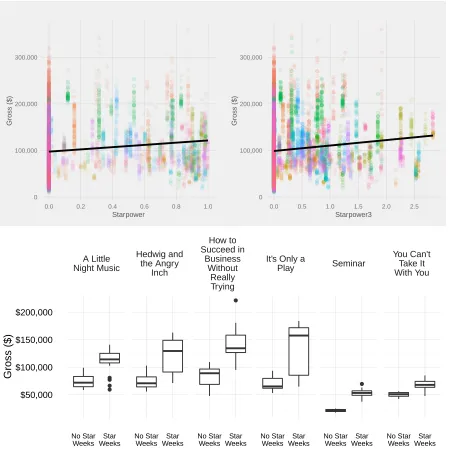
Our main research question concerns how star power effects revenues on Broadway. We first begin with a graphical analysis. In Figure 2.7 we show scatterplots ofGrossagainstStarpower
2.4. Results 19
Table 2.2: Variable Descriptions
Variable Description Data Source
Gross The inflation adjusted, per per-formance revenue for a given show in a given week.
ibdb.com
Starpower The max adjSTARmeter for the set of actors who were in a given show during a given week.
imdb.com
Starpower3 The sum of the three top adjS-TARmeter for the set of actors who were in a given show dur-ing a given week.
imdb.com
CompetitionStarpower The sum of all other shows’
S tar power that were running during the same week.
imdb.com
TonyAwards The maximum number of Tony Awards won for the set of actors
in showiduring weekt.
ibdb.com
OtherAwards The maximum number of other major awards for the set of
ac-tors in showiduring weekt.
imdb.com/grammy.com
DaysOpen Variable indicating how many days the show had been open by
the end of weekt.
N/A
Month Dummy variables indicating whether the last day of the week was in a given month.
N/A
Holiday Dummy variables indicating whether a given holiday occured during the week.
N/A
Table 2.3: Correlation Matrix
Gross Starpower Starpower3 CompetitionStarpower TonyAwards
Gross
Starpower 0.14
Starpower3 0.12 0.91
CompetitionStarpower -0.03 -0.02 -0.02
TonyAwards 0.07 0.38 0.49 -0.02
Table 2.4: Summary Statistics of Variables
Statistic N Mean St. Dev. Min Max
Gross 9,420 102,301.100 56,578.950 10,079.130 360,051.900
Starpower 9,420 0.199 0.333 0.000 1.000
Starpower3 9,420 0.289 0.571 0.000 2.831
CompetitionStarpower 9,420 5.682 1.898 0.160 10.786
TonyAward 9,420 0.154 0.526 0 5
OtherAwards 9,420 0.200 0.843 0 18
on less star power.
To partially deal with this issue, in the second row of Figure 2.7 we provide selected show’s box plots conditional on if a star was present or not that week. We define a “star week” as any show-week combination where S tar power ≥ C whereC is some prespecified constant indicating at what level an actor is considered a star. Here, we assumed thatC = 0.90. In this way we start to control for unobservable individual time-invariant effects.
We see that for the most part there is a difference in behavior between star weeks and no star weeks, with all selected shows reporting higher median gross under a star week than a no star week. Indeed, the effect is visibly apparent.
We can also examine the overall distribution ofGrossconditional on the presence of a star. We then examine the distribution of Grossduring star-weeks as compared to non star-weeks.
14
Our analysis is sensitive to the choice ofC, and thus we provide multiple values to test. We try the following values for C: 0.50,0.70,0.90,0.95. In Figure 2.8, we provide these conditional distributions. Along the x-axis is the specific gross, and along the y-axis is a smoothed estimate of the probability density of a star (green) vs non-star (red) of being at that value. The smoothing was done via a kernel density estimate with a Gaussian smoothing kernel. Bandwidth was selected using Silverman’s rule of thumb. In Table 2.5, we provide the associated mean values of star vs non-star weeks at each definition.
Table 2.5: Mean Values for Star Weeks compared to Non Star Weeks
C Mean / Standard Deviation of Gross during
Star Weeks
Mean / Standard Deviation of Gross during
Non-Star Weeks
0.5 $114,570 (52,394.7) (N=1,993) $99,008.9 (57,207.4) (N=7,427)
0.7 $114,684 (54,913.5) (N=1,498) $99,959.7 (56,588) (N=7,922)
0.9 $99,254.7 (40,467.1) (N=677) $102,537 (57,634) (N=8,743)
0.95 $112,293 (39,590.8) (N=317) $101,953 (57,049.6) (N=9,103)
A few points of interest arise. At all star definitions, the distribution of star grosses appears to be have less variance than the distribution of non-star grosses. This graphical intuition
2.4. Results 21
0 100,000 200,000 300,000
0.0 0.2 0.4 0.6 0.8 1.0
Starpower
Gross ($)
0 100,000 200,000 300,000
0.0 0.5 1.0 1.5 2.0 2.5
Starpower3
Gross ($)
A Little Night Music
Hedwig and the Angry
Inch
How to Succeed in
Business Without
Really Trying
It's Only a
Play Seminar
You Can't Take It With You
$50,000 $100,000 $150,000 $200,000
No Star Weeks
Star Weeks
No Star Weeks
Star Weeks
No Star Weeks
Star Weeks
No Star Weeks
Star Weeks
No Star Weeks
Star Weeks
No Star Weeks
Star Weeks
Gross ($)
Figure 2.8: Distribution of Gross conditional on star presence. Densities estimated via a kernal density estimate, with a Gaussian smoothing kernel. Bandwidth was selected using Silverman’s rule of thumb.
0e+00 5e−06 1e−05
0 100,000 200,000 300,000 GROSS ($)
Density
C = .50
0e+00 5e−06 1e−05
0 100,000 200,000 300,000 GROSS ($)
Density
C = .70
0e+00 5e−06 1e−05
0 100,000 200,000 300,000 GROSS ($)
Density
C = .90
0e+00 5e−06 1e−05
0 100,000 200,000 300,000 GROSS ($)
Density
C = .95
2.4. Results 23
is confirmed by checking the standard deviation of the distributions in Table 2.5. At all C
definitions, the standard deviation of star weeks are less than non-star weeks. In addition, in all but one definition, the mean of star weeks is higher than non-star weeks. Finally, under all definitions, the no-star distribution appears to have a higher probability of achieiving relatively low gross amounts. This would seem to bolster the claim that stars help producers reduce risk. We can also qualitatively examine stochastic dominance of one distribution over the other. In this setting, stochastic dominance exists if, at every potential gross dollar amount, a dis-tribution has at least the probability as the other of achieving a higher gross. Managerially, stochastic dominance would that there is no “downside” to hiring a star as they would have less down-side risk and higher upside risk. At theC =0.50 andC = 0.70 definition, there seems to exist stochastic dominance of stars over no-stars. At other definitions however, there is a clear violation in the upper tail. For example, atC= 0.90 andC =0.95 the non-star distribution has a higher probability of achieving higher grosses This would imply a tradeoff- stars may reduce downside risk but limit upside risk.
2.4.2
Regression Results
The prior sections provide some insights into how stars play a role in a show’s revenue. How-ever, we did not control for show-specific and time-specific effects. Here we provide formal re-sults from multiple fixed-effects regressions and discuss managerial intepretations. Our model aims to predict the log of Gross as a function of star power, award covariates, and various controls. We use show-specific dummy variables to account for any unobserved time-invariant show-specific effects that may exist. These effects might include the script quality, song quality, and budgets.
In Models 1 and 2, we use theStarpowervariable as our measure of star power. In Model 3 and 4 we instead use the ensemble measurement Starpower3. In Models 2 and 4, we add
CompetitionStarpowerto test the effects of competition, but leave it out in Models 1 and 3. We attempted squared terms on theStarpowerandStarpower3variable but only found significance with Starpower3. We thus only report this variable, but present all attempted models in the appendix.
2.4.3
Model Results
In Table 2.6, we present coefficient estimates (and accompanying standard errors), and R2
values from these models.
First, we examine our main research question and variable of interest. Starpoweris positive and statistically significant at traditional levels (5%) across all specifications. The coefficient of
Starpower3is positive and significant on the squared term but insignificant on the main term. This is consistent with the hypothesis that adding star power improves revenues. The positive and significant squared term would indicate increasing returns to ensembles of stars. Note that the two models using theStarpower3variable as a measure of star power have a higher adjusted
R2value, indicating a better fit.
Table 2.6: Regression Results
(1) (2) (3) (4)
Starpower 0.095∗∗ 0.096∗∗
(0.038) (0.037)
Starpower3 −0.055 −0.054
(0.054) (0.053)
Starpower32 0.118∗∗∗ 0.117∗∗∗
(0.028) (0.028)
CompetitionStarpower −0.004 −0.004
(0.006) (0.006)
TonyAwards 0.052 0.014 0.051 0.014
(0.033) (0.035) (0.032) (0.034)
OtherAwards 0.040∗∗
0.021∗
0.039∗∗
0.020∗
(0.017) (0.012) (0.017) (0.012)
DaysOpen −0.411∗∗∗ −0.417∗∗∗ −0.403∗∗∗ −0.409∗∗∗
(0.103) (0.098) (0.102) (0.097)
DaysOpen2 0.031∗∗∗
0.032∗∗∗
0.031∗∗∗
0.031∗∗∗
(0.010) (0.010) (0.010) (0.010)
Constant 12.801∗∗∗
12.796∗∗∗
12.775∗∗∗
12.770∗∗∗
(0.425) (0.416) (0.420) (0.411)
Mean Squared Error 0.03952 0.0381 0.03948 0.03806
Observations 9,420 9,420 9,420 9,420
R2 0.888 0.892 0.888 0.892
Adjusted R2 0.884 0.888 0.884 0.889
Residual Std. Error 0.202 (df=9131) 0.198 (df=9130) 0.202 (df=9130) 0.198 (df=9129)
Note: ∗p<0.1;∗∗p<0.05;∗∗∗p<0.01
Dependent variable of LOG(Gross). Control Variables Excluded. Cluster Robust Standard Errors shown in parentheses.
TonyAwards is positive but not statistically different from zero across all specifications. This is a surprising finding because other major awards do appear to have an effect. To the extent the broadway customer base values success on broadway specifically, we would expect that signals of that success to matter. Awards on Broadway, as a signal of quality, would signal to insiders (and maybe outsiders) that a show is good.
Competitor casting choices, and their effects can also be evaluated with our model. Com-petitionStarpower is negative as predicted, but non-significant across both models. That is, we cannot reject the null hypothesis that competitor casting choices have no effect on a given show. If this hypothesis were true, it would be consistent with the idea that star power attracts consumers who otherwise would not have gone to a Broadway show at all. We discuss the managerial and industry implications of this later in the paper.
Finally, we can estimate the revenue gain from increasing the star power associated with a show. This would be the most managerially relevant outcome from our model, since it would inform whether a blockbuster strategy is likely to pay off. Because of the log transformed dependent variable, to find the average change ofGrossfrom a change inStarpower, we can evaluate the following expression
∆Gross
∆Starpower =Gross
eβ∆Starpower−1
whereβis the estimated coefficient(s) forStarpower.
In our first comparison we examine how our models suggest an average show’sGrosswould improve if the show hired a star actor (adjSTARmeter=0.98) when it previously had no actors with star power(adjSTARmeter= 0). This action would imply an increase in Starpower and
2.4. Results 25
Table 2.7: Estimated effects from hiring single actor with adjSTARMeter=0.98
Specification Average Percent Change Mean Estimate
Model 1 9.8 % $9,983 ($79,868 per week.) Model 2 6.1 % $6,223 ($49,786 per week.) Model 3 9.8 % $10,058 ($80,465 per week.) Model 4 6.2 % $6,300 ($50,403 per week.)
Table 2.8: Estimated effects from hiring two actors with adjSTARMeter=0.7 each
Specification Average Percent Change Mean Estimate
Model 1 6.9 % $7,036 ($56,285 per week.) Model 2 17 % $16,975 ($135,801 per week.) Model 3 6.9 % $7,087 ($56,700 per week.) Model 4 17 % $17,073 ($136,585 per week.)
range from $6,223 in Model 2 to $10,058 under Model 3. Generally, the models built on the ensemble variable predict lower increases for a single star hiring.
We can also explore ensemble star hiring. Instead of hiring a single actor, we consider the estimate effects if a show hired two star actors each with an adjSTARmeterof 0.7. Here, the increase inStarpoweris only 0.7, however the increase inStarpower3is 1.4. We summarize each model’s predicted effects in Table 2.8. Perhaps intuitively, our measure built specifically for ensemble effects predicts a much larger effect than the measure that only measures the top actor. Model 2 predicts a $16,975 average increase in Gross as compared to a $7,036 from Model 1.
2.4.4
Model Diagnostics
We must test that our model assumptions are valid. One key model assumption we made is to treat unobserved individual effects as fixed effects. The theoretical reason is that we did not want to assume that the vector of covariates was independent from the unobserved individual effect. However, we also checked for this assumption via a Hausman Test which confirmed a fixed effects specification (p<2.2e−16)15.
In Figure 2.9, we provide histograms as well as Q-Q plots of the residuals of each of our models. Residuals appear to be normally distributed and centered around zero for all models.
Recall that in our estimation procedure we adjust the standard errors using “cluster robust standard errors”. The Cameron et al. (2011) method is robust to serial correlation and het-eroskedasticity (Wooldridge, 2002, p.275). Our data shows signs of both issues. A Breusch-Godfrey test for serial correlation in panel models finds statistically significant (p < 2.2e−16)
evidence of serial correlation in the residuals. A Breusch-Pagan test for heteroskedasticity also finds significant evidence (p<2.2e−16) against homoskedasticity16.
2.4.5
Case Studies
In the following sections we provide case studies of specific star entries and exits into Broad-way shows. These examples are intended to provide understanding of the business environ-ment. They are also intended to show how practitioners can estimate the effect of a specific star entry. This may be of interest for managers interested in determining post-hoc whether a cast change was worthwhile.
American Idiot
American Idiot was a Broadway musical based on the Green Day album of the same name.
The show opened in April 2010. On September 27, 2010, the show’s producers announced that Green Day lead singer Billie Joe Armstrong would star as the “St. Jimmy” character for only one week, starting only a few days later. After his initial run week run he later played the same characters multiple weeks throughout January and February. On March 10th, 2011 the show announced that it was closing on April 24th and announced even more weeks with the star.
The process of choosing Armstrong for this specific musical was obviously endogenous to the show. The producers chose him due to his connection with the source material. However, the actual weeks chosen was closer to an exogenous process. Unlike most actor contracts on Broadway, the star was in the show in non-contiguous weeks, sometimes with significant breaks. This occured due to the star’s previously scheduled tour and logistical availability. Thus, the choice of which specific weeks the star would be in was constrained.
Table 2.9: Summary Statistics of American Idiot Grosses. Star Weeks are defined as those which included Billie Joe Armstrong.
Star Weeks Non-Star Weeks
Min 83,190 51,930
1st Quartile 118,300 60,460 Median 129,300 65,940 Mean 132,100 66,310 3rd Quartile 149,300 70,100 Max 179,700 83,090
We first separate weeks with and without the star. We label these star weeks and non-star weeks respectively. Summary statistics of these weeks are presented in Table 2.9. There is a difference in means of $65,829 , a statistically significant difference.
This difference could be explained via three mechanisms. The most obvious mechanism is that the star increased awareness or quality of the show in the eyes of consumers. This would
2.4. Results 27
−4 −2 0 2 4
−1.0 −0.5 0.0 0.5 Q−Q Plot Theoretical Quantiles Model 1 Sample Quantiles
Histogram of Residuals
Residuals
Frequency
−1.0 −0.5 0.0 0.5
0
500
1000
1500
2000
−4 −2 0 2 4
−1.0 −0.5 0.0 0.5 Theoretical Quantiles Model 2 Sample Quantiles Residuals Frequency
−1.0 −0.5 0.0 0.5
0
500
1000
1500
2000
−4 −2 0 2 4
−1.0 −0.5 0.0 0.5 Theoretical Quantiles Model 3 Sample Quantiles Residuals Frequency
−1.0 −0.5 0.0 0.5
0
500
1000
1500
2000
−4 −2 0 2 4
−1.0 −0.5 0.0 0.5 Theoretical Quantiles Model 4 Sample Quantiles Residuals Frequency
−1.0 −0.5 0.0 0.5
0
500
1000
1500
2000
Figure 2.10: American Idiot performance relative to control group. Red shading indicates when the star was in the show. Green shading indicates when the public knew there were future performances with the star.
−50% 0% 50% 100% 150% 200%
Oct Nov Dec Jan Feb Mar Apr May
Date
Gross as % of Control Group
Star in the show
Known Future Star Presence
be consistent with the blockbuster strategy and suggest that the star was successful in bringing in additional revenues.
Alternatively, the difference could be due to seasonal time effects. That is, the star being in seasonally “better” weeks, and being associated with an increase without being the cause. In this case study, the likelihood of this mechanism is mitigated because of the constrained process by which weeks were selected. If concert sales and theatre sales are correlated we would expect the star to be in worse weeks, because the “better” dates were taken up by the tour.
Finally, the difference in means could be explained by a temporal altering of purchase by consumers, rather than new consumers. That is, a customer already interested in seeing American Idiot might change the date they see the show to see the star. If so, we would still find a week to week change and association between the star and revenue, but total revenue would be unaltered.