Solar Measurements for 21 cm Wavelength Using 3 m Radio
Telescope
Uday E. Jallod* and Kamal M. Abood
Abstract—Solar hydrogen line emission has been observed at the frequency of 1.42 GHz (21 cm wavelength) with 3 m radio telescope installed inside the University of Baghdad campus. Several measurements related to the sun have been conducted and computed from the radio telescope spectrometer. These measurements cover the solar brightness temperature, antenna temperature, solar radio flux, and the antenna gain of the radio telescope. The results demonstrate that the maximum antenna temperature, solar brightness temperature, and solar flux density are found to be 970 K, 49600 K, and 70 SFU respectively. These results show perfect correlation with recent published studies.
1. INTRODUCTION
Most of the radio data obtained from distant objects like stars, galaxies, pulsars, and quasars are useful for studying the universe. One of the important radio data is the hydrogen line emission at 21 cm wavelength, and this line has different applications in radio astrophysics [1]. This line arises from transitions between the hyperfine structure levels in the ground state of the hydrogen atom. A lot of radio emissions especially from the sun have been studied over decades [2]. Also, many empirical models have been proposed for the solar atmosphere based on spectral lines emissions using Very Large Array (VLA) [3]. Solar radio observations at frequency of 1.42 GHz (equivalent 21 cm wavelength) provides valuable information on the structure and dynamics of the solar atmosphere. At this frequency, we could measure the solar brightness temperature, solar radio flux, and understanding the basic of the physical processes operating in quiet and active regions of solar atmosphere [4]. Most of the solar radio waves originate from the chromosphere and corona. The propagation of these radio waves depends basically on the index of refraction in these layers. Each value of the index of refraction is related to an electron density and a critical frequency. If this frequency of the solar atmosphere below this critical frequency, then the propagation becomes impossible and vice versa [5].
One of the important issues is the solar brightness temperature at centimeter wavelengths measured by different technical methods. Since 1960, the first published studies determined the brightness temperature of the quiet sun at 21 cm wavelength. The technique that has been used for that study is an aerial system which consists of two long arrays, each made up of 32 steerable and spaced by 12.2 m apart on a 380 m base line [6]. In 1968, another paper measured the brightness temperature of quiet sun at centimeter, millimeter, and infrared wavelengths [7]. Solar observations were made with a single dish of 27 m diameter using frequency — agile receiver at 20 frequencies over the range 1.4 to 18 GHz by Zirin et al. [8]. Many authors have made compilations of the solar brightness temperatures at microwave and millimeter ranges by different observation techniques [9]. The development of the interferometry technique leads to recording the first solar radio image at Kit Peak National observatory using 21 cm wavelength [10].
Received 10 April 2019, Accepted 22 May 2019, Scheduled 12 June 2019
* Corresponding author: Uday E. Jallod (udayjallod@scbaghdad.edu.iq).
Nowadays, solar radio physics is one of the most rapidly developing fields of astrophysics after developing the observational facilities such as Chinese Spectral Radio Heliograph (CSRH), Siberian Solar Radio Telescope (SSRT), and Atacama Large Millimeter/Submillimeter Array (ALMA) [11]. Other observing systems are used to observe solar radio emissions, and one of the most important observing systems is a broadband radio spectrometer. It plays an important role in observing and revealing the physical processes of the solar atmosphere. There are several solar broadband radio spectrometers running in the world, such as Phoenix at ETH Zurich (100–4000) MHz, Ondrejov Radio Spectrograph in the Czech Republic (800–5000) MHz, and Brazil broadband spectrometer (200–2500) MHz. All the above spectrometers are single dish telescopes which receive the radio emission of the full solar disk without spatial resolution [12].
2. METHODOLOGY
2.1. Theoretical Concepts
The Plank’s law for blackbody radiation is given by [13]:
B = 2hv 3
c2
1
ehv/kT −1 (1)
whereB is the brightness (intensity of specific frequency) measured in (W/m2/Hz/rad2),hthe Planck’s constant (Joule. second), v the frequency in Hz, k the Boltzmann constant (Joule/K), c the speed of light, andT the source temperature in K.
In the centimeter wavelengths regions (hvkT), this provides the Rayleigh-Jeans approximation for blackbody radiation at radio wavelength (λ) [13]:
B = 2KT v 2
c2 2kT
λ2 (2)
The concept of the antenna temperature (TA) could be defined as the temperature of antenna radiation resistance, which equals resistance temperature. TA is created due to the relation between the power radiated by the source, which is associated with the brightness temperature TB, and the antenna normalized power pattern P(θ,Φ). Consider a receiving antenna that is pointed at a source brightness distributionB(θ,Φ) when the source power radiated intercepted by the antenna terminals creates power called antenna powerPA. TAis associated withPAat antenna radiometer, andPAcould be given by [14]:
PA= 12Ae B(θ,Φ)P(θ,Φ)dΩ (3)
where (θ,Φ) are the azimuth and elevation of the source. Ae is the effective aperture of the radio telescope antenna, and dΩ is the element solid angle. Utilizing Raleigh-Jeans limit. Therefore, the brightness distribution given by Eq. (3) can be changed by an equivalent TB, andTA can be given by the following equation [14]:
TA= 1
2kAe TB(θ, φ)P(θ, φ)dΩ (4)
This means that TA is equivalent to the convolution between the source brightness temperature and beam power pattern of the radio telescope. Using the Nyquist theorem can introduceTA by [15]:
TA= PA
kΔv (5)
where Δv is the bandwidth frequency of the telescope radiometer in Hz.
In the case of the solid angle Ωs subtended by the source is much larger than the solid angle subtended by the antenna ΩA, and this leads to assuming thatTA is exactly equal toTB. If the source does not completely fill the beamwidth, i.e., ΩAΩs, the measured TA will be less than TB, then TB is given by [15]:
TB= ΩA
ΔTAcan be written as [16]:
ΔTA=TAon−source −TAoff−source (7)
Eq. (7) represents the subtraction between TAon−source due to the observed source and TAoff−source due to the sky background.
For a discrete radio source of temperature T and a source solid angle Ωs, the source flux density (s) in Rayleigh-Jeans limit is obtained by integration over the source Ωs [17]:
s=
2kTBv2
c2 dΩ (8)
IfTB of the source is uniform across Ωs, this is reduced to [18]:
s= 2kTB
λ2 Ωs (9)
The observed radio flux density of the source can be written in terms ofTA as [18]:
s= 2kTA
λ2 ΩA (10)
Eq. (9) and Eq. (10) are equivalent. Equation (10) can be written as:
s= 2kTA
Ae (11)
The real observed solar flux density (so) should subtract the contribution of the sky background (ssky) as given by [19]:
so=s−ssky (12)
wheres is the flux density on the surface of the sun.
2.2. Observations and Data Reduction
The 3 m University of Baghdad radio telescope is used to observe the sun in this study. This telescope has focal length of 1 m, 5 degrees beamwidth, and 3.7 degrees of Half Power Beam Width (HPBW) which represents ΩA measured by sun drift scan technique [20]. Aperture efficiency of this telescope (η) is (0.54) measured by observing Cassiopeia-A source [21]. First of all, any radio telescope should be calibrated before any process of observation. Our telescope has been calibrated using the sun and the moon as a reference source. This calibration is applied to two methods including antenna position and radio detector calibrations [22]. This telescope can make daily measurements of the radio signals at the frequency of 1.42 GHz. The spectrometer software of this telescope divides the received data into 600 channels of the frequency. These channels are used to obtain the amplitude of the measured power in unit (dBm). The values of this power are divided according to the frequency channels and arrangements as rows data. This power has been obtained after setting the optimum values of spectrometer parameters of the radio telescope. These parameters are span, sweep time, center frequency, Resolution Bandwidth (RBW), and Video Bandwidth (VBW).
The best solar observations are recorded using spectrometer parameters as listed in Table 1.
Table 1. Selecting spectrometer parameters values.
Source Date Local Time Input Value of
Spectrometer Parameters
Sun 30-12-2018 12:02
Noon Freq. (Hz)Center Time (Sec.)Sweep Span(Hz) RBW(Hz) VBW(Hz)
Noise
Background 21-1-2019
6.06
Night 1.42×10⁹ 30 2×10⁷ 105 10
the sun remains within the beamwidth. Sky background noise is estimated after the sunset (the sun is completely disappeared). This estimation is then subtracted from our observation in order to avoid unwanted noise error. It should be pointed out here that the sky background noise is also recorded within 5 minutes in order to maintain the signal and noise observations in the same size.
3. THE RESULTS AND DISCUSSIONS
Our telescope saves the observed radio data into a notepad sheet and then transferred to Excel. This sheet is imported to the MATLAB environment to implement many processes such as the conversion units of the observed power data, applying most equations that are listed in the theoretical section, and displaying the results. All the results of this article are plotted as a function of frequency in order to reveal the quality of the radio telescope at the center frequency of our detector (1.42 GHz).
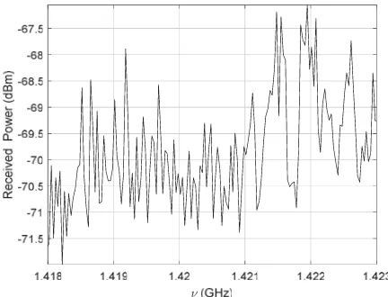
Figures 1 and 2 demonstrate the received power as a function of frequency for the sun and sky background noise, respectively.
Received Power (dBm)
Figure 1. Received power (dBm) as a function ofv (GHz) (date Dec. 30, 2018).
Figure 2. Received sky background power (dBm) andv (GHz) (date Jan. 21, 2019).
The center portion of Figure 1 is extracted, and a Gaussian function is then made to fit the observed data. The quality of fitting is verified by using Cross Correlation Coefficient (CCC) criterion [23]:
CCC= σxy
σxy = N1
N
i=1(xi−mx)(yi−my) (14)
where x and y represent the received power data and fitted data, respectively. σxy is the standard deviation for both real and fitted data. σx and σy are the standard deviations of the observed power data and fitted data, respectively. mx is the mean value of the observed power data, and my is the mean value of the fitted data. N is the number of frequency channels (here N = 600 channels).
The optimum value ofCCC that verifies the fitting Gaussian function, shown in Figure 3, is found to be 0.799. This value shows high correlation between the observed and fitted data.
Figure 3. Real data (solid line) and its Gaussian fitting (o-).
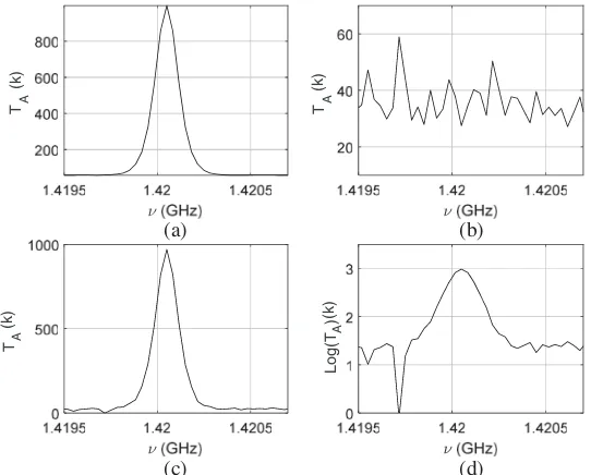
The received powers for the sun and sky background are converted to the temperatures (K) via Eq. (5) using k = 1.38×10⁻²³ (Joule/K) and Δv = 2×10⁸Hz. The measured TA due to the sky background is then subtracted from the measured TA due to the sun via Eq. (7).
The results are shown in Figure 4.
TA
(k)
TA
TA
(a) (b)
(c) (d)
(k)
(k)
Log(T )
A
(k)
The logarithmic scale is used to reduce the dynamic range between the values ofTAand gives more details about the behavior of the curve. A sharp transition reaches zero due to the subtraction which means that TA for the sun and sky background are equal at this point, as shown in Figure 4(d).
TB is computed according to Eq. (6), using Ωs = 0.5◦, ΩA = 3.7◦. The results are shown in Figure 5.
(a) (b)
Figure 5. (a)TB (K) as a function ofv (GHz), (b) logarithmic scale of (a).
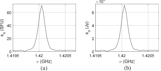
The observed solar flux density is computed in two units via Eq. (12). The first is the Solar Flux Unit (SFU), and the second is the Jansky (Jy). Using SFU = 104 Jy or SFU = 10−22W·m−2Hz−1 and Jy = 10−26W·m−2Hz−1.
The results are illustrated in Figure 6.
(a) (b)
Figure 6. (a)so (SFU) as a function of v (GHz), (b)so (Jy) as a function of v (GHz).
These computed results are compared with Natural Resources Canada [24], Jodrell Bank Internet Observatory of Manchester University, and the values of TA, TB are compared with MIT Haystack observatory reports [25].
Finally, the gain (G) of the reflected parabolic antenna can be defined as the ability of the antenna to transform the available power at its input terminal to the radiated power. This quantity is used to measure the total power radiated by the antenna in practice. Our antenna gain is computed as follows [30]:
G= 10 log10
4πA λ2 η
(15)
where A is the geometrical area of the radio telescope antenna (m2) for our telescope (A = 7.06 m2), and η is the aperture efficiency. η can be obtained from the surface integral of the radiated power (pr) over the radiation sphere divided by the input power (po). ηis a measure of the relative power radiated by the antenna to the input power as given by [27]:
η= pr po
2π
0
π
0
G(θ, φ)
and can be given as [27]:
η= Ae
A (17)
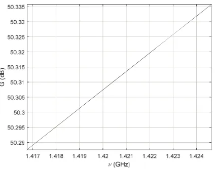
The antenna gain against the frequency is computed according to Eq. (15) as shown in Figure 7.
G (dB)
Figure 7. G(dB) as a function ofv (GHz).
Gis approximately constant with a little increment over the concentrated region of the frequency by the radio detector of our telescope.
4. CONCLUSIONS
Several important points can be extracted from the results of this study.
1. The rad1io telescope spectrometer parameters are crucial parameters that control the observed signals. These parameters are considered primarily responsible for revealing the observed signal from the noise level. The best values of these parameters have been selected depending on empirical attempts, as displayed in Table 1.
2. Maximum value ofTAis 970 K. This value has been determined according to the strength measured power of the sun, as shown in Figure 4.
3. Total TB profile has been measured and found to be equal to 49600 K. This value is computed from Figure 5 by taking the summation for all values ofTB inside ΩA. TB value is considered very promising result because it is in a perfect correlation with recent published results.
4. Maximum of so is measured at a time of observation and found to be equal to 70 SFU or 7×10⁵ Jy according to the peaks shown in Figure 6.
5. G has a slight increment with the increment of the frequency and is approximately equal to 50.307 dB at 1.42 GHz as illustrated in Figure 7.
ACKNOWLEDGMENT
We would like to express our thank and gratitude to the head of the Department of Astronomy and Space, academic staff, colleagues and all friends at the College of Science, University of Baghdad for their valuable advices and encouragement.
REFERENCES
2. Usoslin, I. G., “A history of solar activity over millennia. Living rev.,” Solar Physics, Vol. 5, No. 3, 6–19, 2008.
3. Sehorst, C. L., A. V. Silva, andJ. E. Costa, “Solar atmospheric model with spicules applied to radio emission,”Astronomy and Astrophysics, Vol. 433, 365–374, 2005.
4. Shibasaki, K., C. E. Alissandrakis, and S. Pojolainen, “Radio emission of the quiet sun and active regions,”Solar Physics, Vol. 273, 309–337, 2011.
5. Labrum, N. R., “The radio brightness of quiet sun at 21 cm wavelength near sunspot maximum,”
Australia Journal Physics, Vol. 13, 700–711, 1960.
6. Krishnan, T. and N. R. Labrum, “The radio brightness distribution on the sun at 21 cm from combined eclipse and pencil-beam observation,”Australia Journal Physics, Vol. 14, 403–419, 1961. 7. Shimabukuro, F. I. and J. M. Stacey, “Brightness temperature of the quiet sun at centimeter and
millimeter wavelengths,” The Astrophysical Journal, Vol. 152, 777–782, 1968.
8. Zirin, H., B. M. Baumert, and G. J. Hurforf, “The microwave brightness temperature spectrum of the quiet sun,”The Astrophysical Journal, Vol. 370, 779–783, 1991.
9. Kuseki, R. A., “The solar brightness temperature at millimeter wavelength,”Solar Physics, Vol. 48, 41–48, 1976.
10. Dulk, G. A. and D. E Gary, “The sun at 1.4 GHz: Intensity and polarization,” Astronomy and
Astrophysics, Vol. 124, 103–107, 1983.
11. Nakariakov, V. M., L. K. Kashapova, and Y. H. Yan, “Editorial: Solar radiophysics-recent results on observations and theories,” Research in Astronomy and Astrophysics RAA, Vol. 14, No. 7, 1–6, 2014.
12. Tan, C., Y. Yan, B. Tan, Q. Fu, Y. Lin, and G. Xu, “Study of calibration of solar spectrometer and the quiet sun radio emission,” The Astrophysical Journal, Vol. 808, No. 61, 21–41, 2015. 13. Wilson, T. L., K. Rohlfs, and S. Huttemeister, Tools of Radio Astronomy, 6th edition,
Springer-Verlag Berlin Heideelberg, 2013.
14. Ptatap, P. and G. Mclntosh, “Measurements of the radiation from thermal and non thermal radio sources,”American Association of Physics Teachers, Vol. 73, No. 5, 399–404, 2004.
15. Neil, K. O., “Single dish calibration techniques at radio wavelength,” Astronomical society of the
Pacific ASP Conference Series, Vol. 278, San Francisco, CA, 2001.
16. Saha, S. K., Diffraction-limited Imaging with Large and Moderate Telescopes, World Scientific Publishing Co. Pte. Ltd, 2007.
17. Pacini, A. A. and J. P Raulin, “Solar radio emission,”Advances in Space Research, Vol. 35, 793–754, 2005.
18. Gary, D. and C. Keller, Solar and Space Weather Radio Physics Current Status and Future
Developments, Springer Science + Business Media, INC, 2005.
19. Kalinov, V., “Solar observations with the small radio telescope,”Bulgarian Astronomical Journal, Vol. 15, 107–112, 2011.
20. Zaineb, A. J. and K. M. Abood, “Study of some parabolic radio telescope antenna parameter,”
Iraqi Journal of Science, Special issue, Part B, 453–461, 2016.
21. Hoobi, M. R. and K. M. Abood, “Calibration of a three meter small radio telescope in baghdad university using the sun as a reference source,” Iraqi Journal of Science, Vol. 60, No. 1, 171–177, 2019.
22. Abood, K. M. and A. M. Kitas, “Background radio emissions at 1.42 GHz,”Iraqi Journal of Science, Vol. 59, No. 2A, 786–791, 2018.
23. Goodman, J. W., Statistical Optics, John Willy & Sons, Inc., New York, 2000. 24. http://www.spaceweather.gc.ca/sx-11-eng.php.
25. Massachusetts Institute of Technology Haystack Observatory.
26. Milligan, T. A.,Modern Antenna Design, 2nd edition, A John Wiley & Sons, Inc., 2005.