Efficient Bayesian Multifidelity Approach in Metamodeling
of an Electromagnetic Simulator Response
Tarek Bdour1, 2, *, Christophe Guiffaut1, and Alain Reineix1
Abstract—Several computer codes with varying accuracy from rigorous full-wave methods (high-fidelity models) to less accurate Transmission Line (TL) approaches (low-(high-fidelity model) have been proposed to solve EMC problems of interference between parasitic waves and wired communication systems. For solving engineering tasks, with a limited computational budget, we need to build surrogate models of high-fidelity (HF) computer codes. However, one of their main limitations is their expensive computational time. Rather than using only the computationally costly HF simulations, we apply another type of surrogate models, called Multifidelity (MF) metamodel which efficiently combines, within a Bayesian framework, high and low-fidelity (LF) evaluations to speed up the surrogate model building. The numerical results of combination of an expensive EMC simulator and a cheap TL code to solve a plane wave illumination problem, show that, compared to Kriging, a reliable Bayesian MF metamodel of equivalent or higher predictivity can be obtained within less simulation time.
1. INTRODUCTION
The analysis of the coupling between high-frequency electromagnetic fields and conducting wires has become a primary issue in EMC domain, due to various sources of electromagnetic field that can impact the devices connected by power or signal transmission lines.
The problem of electromagnetic field-to-line coupling can be solved by using different approaches that can be classified into two main categories with respect to their complexity: the classical transmission line (TL) theory [1] and full-wave methods.
The full-wave approach based on Method of Moments (MoM) and implemented in Numerical Electromagnetic Code (NEC-2) [2] is one of the well adapted approaches to solve the field-to-line problem in both low and high frequencies. However, when electrically long or high lines are involved, NEC-2 simulator becomes very time consuming, which penalizes the numerical cost to build a surrogate model with a reasonable accuracy. Multifidelity surrogate (MFS) models have been developed to compensate for inadequate expensive high-fidelity data with cheap low-fidelity data by modeling the connection between them.
The last two decades have seen a major increase in publications on multifidelity methods for computational design. These methods use two types of models for the evaluation of designs: the high-fidelity model (HF) provides the reference in terms of accuracy and the low-high-fidelity (LF) models produce less accurate response values, but at significantly lower expense.
Space Mapping (SM), initiated in [3], is a physical multifidelity method based on a linear transformation (mapping) that makes a coarse model behave as a fine model. In electromagnetics, Koziel and Bandler [4] have used the SM technique to model microwave devices.
Received 1 December 2016, Accepted 19 January 2017, Scheduled 8 February 2017 * Corresponding author: Tarek Bdour ([email protected]).
1 EMC and Diffraction Research Team, Research Institute XLIM, Limoges 87066, France.2Chaire C2M, COMELEC dept,
Relying on the success of the geostatistical technique called kriging [5, 12], the first MFS model based on Gaussian Process (GP) [6] was introduced by Kennedy and O’Hagan [7]. The direct Co-Kriging, introduced by Forrester et al. [8], provides a deterministic formulation for fitting the GP parameters with a non-informative prior. This Co-Kriging approach has been applied in [9] to design metamaterial circuits for optimization purposes. However, the variance of the surrogate response could be underestimated [7].
The Bayesian Co-Kriging model, developed in [10], allows the incorporation of prior information on GP hyperparameters and is based on joint estimation between these hyperparameters. It is important to highlight that this method benefits from good computational characteristics of Bayesian approaches such as having information about the uncertainties of the estimation parameters (through their prior and updated distributions). In [13], the authors have applied a multifidelity Bayesian support vector regression to surrogate the input of planar antenna. To the authors’ knowledge, this work is the first contribution that applies a Co-Kriging based Bayesian multifidelity framework to electromagnetics.
In this article, the direct and Bayesian approaches of MF Co-Kriging will be used to build surrogates models for the EMC computer code, and their numerical performances will also be compared and discussed.
This paper is organized as follows. Section 2 describes the derivation of the transmission line model (LF model). Section 3 gives a brief theoretical background of the multifidelity modeling approach. In Section 4, the adopted multifidelity method is applied to a typical EMC problem, and its efficiency is compared to other metamodeling techniques. Some concluding remarks are provided in Section 5.
2. LOW-FIDELITY MODEL
The aim of this section is to derive a simple Transmission Line model (low-fidelity model) to investigate the radiated susceptibility of a perfect electric conductor (PEC) cable illuminated by an external electromagnetic field.
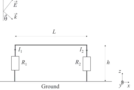
The geometry of the studied EMC problem is illustrated in Fig. 1. A wire of length L and radius ais located over an infinite and perfectly conducting ground at heighthin the presence of a transverse electric (TE) plane wave of amplitudeE0 and incidence angle θ. The terminal resistances between the wire and the ground areR1 and R2.
θ
R1 R2
Ground
L
h
I1 I2
x y z E
k
→ →
Figure 1. Geometry of a PEC line illuminated by a TE plane wave.
Using Baum-Liu-Tesche (BLT) equation [1], the induced currents at the line terminals I1 and I2 can be written in a matrix form as:
I1 I2
= 1
Zc
1−ρ1 0 0 1−ρ2
−ρ1 eγL eγL −ρ2
−1 S1 S2
(1)
When the height of the cable above ground h is no longer electrically small, the field variation along the vertical risers should be taken into account. Then, the excited lumped sources into both vertical risers have to be incorporated in BLT equation. To simplify this latter, the three transmission lines (cable and two risers) are supposed to have the same characteristic impedance Zc, so the wave
propagation can be considered in a single line of effective lengthL+ 2h. The resulting voltage excitation sources are given by [11]:
S1 S2
= E0 2
ejkzh−e−jkzh× ⎡ ⎣
e(γ−jkx)L−1 A
γ−jkx −jBkz
eγLe−(γ+jkx)L−1 (γ+Ajkx)+jkB
z
⎤
⎦ (2)
withA=−cosθ,B= sinθ,kx =ksinθ and kz =−kcosθ.
3. MULTIFIDELITY METAMODELING: BAYESIAN CO-KRIGING
In this section, the theoretical background of Kriging [12] and Bayesian Co-Kriging [10] approaches are described. Only the main properties and equations are provided. For further details, the reader is referred to the mentioned references.
Let us suppose that we want to surrogate an expensive computer code output zs(x) with
x = [x1, . . . , xd]T a vector of d design variables. We assume also that low fidelity versions of this
code (zl(x))l=1,...,s−1 are available. These codes are sorted by order of fidelity from the less accurate z1(x) to the most accurate zs−1(x). Our prior belief is that all code levels zl(x) can be modeled as
realizations of Gaussian processes (Zl(x))l=1,...,s.
For each level l = 1, . . . , s, let define the experimental design Dl ={x1, . . . , xnl} with n
l samples,
such that Ds ⊆ Ds−1 ⊆ . . . ⊆ D1 i.e., ns ≤ ns−1. . . ≤ n1), the vectors of true and approximated responses, respectively zl = [zl(x1), . . . , zl(xnl)]T and Zl = [Zl(x1), . . . , Zl(xnl)]T and the
iteratively-formed sets z(l) = (z1, . . . ,zl) and Z(l)= (Z1, . . . ,Zl).
3.1. Kriging
In this section, we model each computer code zl(x) as a draw from an independent Gaussian process
(GP) distribution [12].
Given the experimental design of nl samples Dl and its corresponding response vector zl, the
Kriging model Zl(x) approximates the true function zl(x) as
Zl(x)∼ GP
μlnl(x), Sl(x)
=μlnl(x) +Sl(x) (3)
where the deterministic functionμlnl(x) =fl(x) Tβ
l is the mean value of the Gaussian process; T stands
for the transpose;βl = [βl0, . . . , βpll]
T is a vector of p
l regression parameters; flT(x) = [f1l(x), . . . , fpll(x)]
is a vector ofplbasis functions; the stochastic model Sl(x), corresponding to the deviation fromμlnl at
x, is defined as the Gaussian random variable N(0, σ2
l), with variance σ2l and a stationary covariance
functionCl(x, x) = Corr[Sl(x), Sl(x)] =σl2Rl(x, x,ϕl). The autocorrelation functionRl describes the
correlation between two samples x andx of the d-dimensional input space, and depends on the vector of hyperparameters ϕl= [ϕl
1, . . . , ϕld]T. It is defined as
Rl(x, x, ϕl) = d
k=1 rlk
xk, xk, ϕlk
(4)
whererlk(xk, xk, ϕlk) is a 1D correlation function along thek-th componentxk of samplex.
One of the popular choices for the correlation function is the Gaussian function, related to the weighed distance between the two corresponding points xand x as
rlk
xk, xk, ϕlk
= exp
−ϕl
kxk−xk 2
ϕlk≥0
(5)
where the hyperparameterϕl
Based on the best linear unbiased prediction (BLUP) [12], the Kriging predicted response at an unobserved pointx∗ is a Gaussian variable Zl(x∗) with meanμlnl(x∗) and variance ˆs
2
l(x∗), defined as
μlnl(x∗) = E[Zl(x∗)|zl] =f T
l βˆl+rTl Rl−1
zl−Flβˆl
(6)
ˆ
s2l(x∗) = V[Zl(x∗)|zl] = ˆσl2
1−rlTRl−1rl+ulTFlTRl−1Fl ul (7)
where the optimal Kriging variance ˆσl2 and the generalized least square regression weights βˆl are respectively given by:
ˆ σl2 =
1 nl
zl−Flβˆl T
R−l 1
zl−Flβˆl
(8)
ˆ
βl =
FTl R−l 1Fl − 1
FTl R−l 1zl (9)
where, for i, j = 1, . . . , nl and k = 1, . . . , pl, Fl = [Fl,ik] = [fkl(xi)] is the design matrix; fl is a vector
whosek-th element isfkl(x∗);Rl= [Rl,ij] = [Rl(xi, xj,ϕˆl)] is the correlation matrix of the experimental
designDl;rlis a vector whosei-th element isrli=Rl(xi, x∗,ϕˆl); the vector of optimal hyperparameters
ˆ
ϕl is obtained through maximum-likelihood estimation.
In summary, to build the model Zs, surrogate of the HF code zs, we start from generating a
random experimental designDs, calculate the vector of its corresponding responseszs by applying the
computer codezs and assume an a priori spatial correlation between design variables (here a Gaussian
correlation functionRsis chosen). After algebraic operations in Eqs. (6) and (7), we can get a
Kriging-based prediction μsns(x∗) on an untried pointx∗, and even more we can get an idea about prediction
uncertainty atx∗ with the mean squared error ˆs2s(x∗). This is the key advantage of Kriging, in opposite
to other metamodels that cannot provide an inherent error measure.
3.2. Co-Kriging Framework
Instead of metamodeling the computer codezs only from its expensive HF evaluations, we manage to
combine it, within a unified Co-Kriging framework, to all of its LFs−1 versions zl(l=1,...,s−1).
Since we have hierarchy ofsresponses, we can use the following autoregressive model proposed by Kennedy and O’Hagan [7]:
⎧ ⎨ ⎩
Zl(x) =ρl−1Zl∗−1(x) +δl(x)
Zl∗−1(x)⊥δl(x)
Zl∗−1(x)∼
Zl−1(x)|Z(l−1)=z(l−1),βl−1,ρl−1,σ2l−1,ϕl−1
(10)
where ρl−1 is the adjustment coefficient between two successive levels l and l−1; ⊥ denotes the independence relationship; δl(x) models the discrepancy between the level l and the adjusted level
l−1. By convention, Z1(x) has the same distribution as δ1(x) (ρ0 = 0).
Forl = 1, . . . , s, conditioning on vectors of regression parameters βl = [βT
1, . . . ,βTl ]T, adjustment
coefficients ρl = [ρ1, . . . , ρl]T, variances σl2 = [σ21, . . . , σl2]T and correlation parameters ϕl =
[ϕT1, . . . ,ϕTl ]T, the discrepancy function δl(x) is modeled as a Gaussian process, starting from the
vector δl(Dl) containing the values ofδl(x) at the points inDl as:
δl(x)∼ GP
flT(x)βl, σl2rl
x, x,ϕl
(11)
From the assumption of conditional independence betweenδl(x) andZl−1(x), . . . , Z1(x) in Eq. (10), we can separately estimate the Co-Kriging hyperparameters{(β1,ϕ1, σ12),(β2,ρ1,ϕ2, σ22), . . . ,(βs,ρs−1,ϕs,
σs2)} to build the s-level model of interest Zs(x), surrogate of the most accurate codezs(x), given all
3.3. Bayesian Estimation of Co-Kriging Hyperparameters
Using Bayes theorem, the probabilities of Co-Kriging hyperparameters, at level l, are updated to a posterior estimation given the probability distributions of their priors and the observation sets
Z(l) =z(l) [10].
Within this Bayesian framework, not only the Co-Kriging parameters are estimated with a deterministic mean value, but also their estimation uncertainties are calculated. In the following, we give the main formulas of posterior hyperparameter estimates using the Bayesian approach.
For all l = 1, . . . , s and thanks to the nested property Dl ⊆ Dl−1, the joint posterior Bayesian distribution of parameters ρl−1 and βl has the following closed form:
ρl−1
βl
∼ NHTl R−l 1Hl −1HTl Rl−1zl, σl2HlTR−l 1Hl −1
(12)
withHl=zl−1(D l)Fl.
For each level l = 1, . . . , s, the variance parameter σ2
l is estimated with a restricted maximum
likelihood method. Its estimate is given by ˆσl2 = (zl−Hl(
ˆ ρl−1
ˆ
βl )) TR−1
l (zl−Hl(
ˆ ρl−1
ˆ
βl ))/(nl−pl−1)
where ( ρˆlˆ−1
βl
) is the mean estimate of ( ρβl−1
l ) in Eq. (12).
The predictive distribution Zs∗(x∗) is not Gaussian. Nevertheless, we can obtain closed form
expressions for its mean μsns(x∗) and variance ˆs2s(x∗) (expression given in [10]).
Finally, the Bayesian Co-kriging-based prediction μsns, resulting from the combination of a HF
code zs and its LF versions (zl)l=1,...,s−1, at an unobserved point x∗ is given by the following iterative relationship for alll= 1, . . . , s:
μlnl(x∗) = ˆρl−1μ l−1
nl−1(x∗) +μδl(x∗) (13)
where
μδl(x) =flT(x) ˆβl+rTl (x)R−l 1
zl−Flβˆl−ρˆl−1zl−1(Dl)
(14)
4. NUMERICAL RESULTS
In this section, a plane wave illumination example is used to demonstrate the characteristics of the Co-Kriging multifidelity surrogate model developed in Section 3. With reference to the geometry described in Fig. 1, a line of lengthL= 8 m, radiusa= 0.01 m, and height above the groundh= 4 m is illuminated by a TE polarized plane wave with amplitude E0 = 1 V/m, at frequency f = 20 MHz. The terminal loads are respectivelyR1 = 50 Ω andR2 = 50 Ω.
Despite its simplicity, this EMC problem is chosen for didactic purposes. In fact, the corresponding high-fidelity simulations can be conducted in a reasonable amount of time in order to numerically and graphically show the advantages of the Bayesian multifidelity technique.
Here, the output of interest is the magnitude of the induced current responseI1on the loadR1. The simulation results are obtained by the proposed analytic BLT model in Eq. (1) (LF model) and full-wave commercial software NEC-2 (HF model). The average CPU runtime of a single NEC-2 simulation is 0.67 s on a 2.6 GHz I7 processor computer with 1 GB of RAM, whereas one BLT simulation takes only 0.52 ms (one LF simulation is 1288 times faster than one HF run).
Our purpose is to build an efficient MF model ˆM(with s= 2 levels) that replaces the expensive NEC-2 codeMand gives accurate predictions for the whole input space. According to the framework in Eq. (10), BLT and NEC-2 simulations are denoted respectively by levels 1 and 2.
Next, we assume uncertainty (due to randomness or engineering design requirements) in the plane wave incidence angle θand the value of the terminal resistanceR1.
4.1. One-Dimensional Problem
HF simulations z2(θi)i=1,...,n2 and a lot of LF simulations z1(θi)i=1,...,n1 obtained by the cheapest code
(BLT equation).
The goal of this section is to compare the numerical performances of metamodels built using Kriging [6], direct Co-Kriging [8] and Bayesian Co-Kriging [10].
To investigate the accuracy of each metamodel, the Mean Relative Square Error (MRSE) of a separate validation dataset is chosen here as a criterion to measure the prediction ability of such
metamodels at non-observed locations. It is defined byM RSE =
1 Nv
Nv i=1
(M(xMi)−(xMˆ(xi)
i) ) 2
, whereNv is
the number of validation samples.
We choose n2 = 6 HF training points (D2) to build the Kriging metamodel of the induced current response. It is worth noting that the relative small budget n2 = 6 is deliberately chosen since it is challenging to any metamodel surrogating the multimodal NEC-2 response illustrated in Fig. 2. The Kriging method is implemented using a Matlab code called DACE [6]. The interpolated Kriging curve
ˆ
MK(θ), using Eq. (6), is illustrated in Fig. 2. Then1= 69 LF training points (D1) are generated using a uniform spatial step Δθ= 2.5◦. We recall here the nested property (D2 ⊂D1) noted earlier.
To build the MFS models, the 6 HF points are combined to the 69 LF points to generate the Bayesian Co-Kriging model ˆMBCoK according to the framework in Eq. (10) and the direct Co-Kriging model ˆMDCoK according to Forrester’s method [8]. Both Co-Kriging curves are plotted in Fig. 2.
The MRSE of each metamodel is computed at Nv = 18 random test samples. The numerical
values of RMSEs are given in Table 1. The resulting relative errors are M RSEBCoK = 0.0258,
M RSEK = 0.0993 and M RSEDCoK = 1.620. This means that, with only 6 HF training points, the
Bayesian Co-Kriging captures the actual behavior of NEC-2 current response better than Forrester’s method and significantly improves the Kriging metamodel. The difference between BCoK and DCoK approaches can be explained by the fact that Bayesian approach takes into account the uncertainties of its estimation hyperparameters while the Direct approach tends to underestimate them.
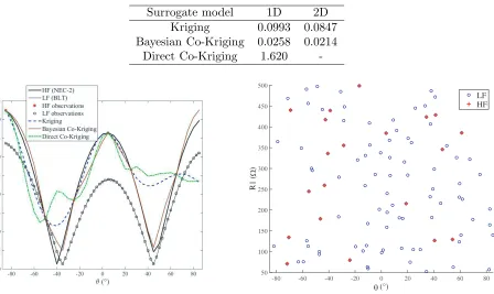
Table 1. RMSEs of surrogate models.
Surrogate model 1D 2D
Kriging 0.0993 0.0847
Bayesian Co-Kriging 0.0258 0.0214
Direct Co-Kriging 1.620
-Figure 2. Metamodeling methods applied to the one-dimensional problem M(θ) =I1(θ).
(°)
-80 -60 -40 -20 0 20 40 60 80
R1 (
)
50 100 150 200 250 300 350 400 450 500
LF HF
θ
Ω
In the next section, the Bayesian approach will be retained as the main MF metamodeling technique.
4.2. Two-Dimensional Problem
In this section, we assume an additional uncertainty in the value of the terminal resistanceR1. Thus, the design variables arex= [θ R1]T, and the design space is defined by−85≤θ≤85◦ and 50≤R1≤500 Ω. For training input data, n2 = 20 HF points and n1 = 116 LF points were randomly selected respecting the nested property (D2 ⊂ D1). The corresponding experimental designs D2 and D1 are depicted in Fig. 3.
Figure 4 depicts the high-fidelity output of the induced currentI1 computed by NEC-2 simulator. As shown in Fig. 5, the Kriging of HF samples fails to accurately predict the output of interest compared to the accurate response in Fig. 4. As shown in Table 1, the MRSE calculated at a validation set of Nv = 100 random samples gives M RSEK = 0.0847, which shows that the 20 HF observation points
are not sufficient to build a metamodel with a good predictivity. However, the same set of accurate observation samples, combined to the 116 low-level samples in the Bayesian Co-Kriging framework in Eq. (10) yields a reliable MF metamodel with a good mean relative error M RSEBCoK = 0.0214.
Moreover, the goodness of fit of the obtained metamodel can be graphically checked by comparing
Figure 4. High-fidelity response surface using NEC-2 simulations.
Figure 5. Response surface of the Kriging metamodel using [6].
Fig. 6 to Fig. 4. Numerical experiences show that we need to add more than 6 HF samples for the Kriging framework [6] in order to obtain the same mean error as the Co-Kriging metamodel, e.g., M RSEK =M RSEBCoK which costs additional runtime of 4.02 s while the overall runtime of 116 LF
simulations is only about 0.06 s (6600% runtime gain). This computational gain highlights the strength of the proposed Co-Kriging framework [10], since it allows us to make good low-cost predictions of the expensive NEC-2 code in a reasonable computational time by efficiently combining both expensive and cheap computer code simulations.
5. CONCLUSION
In this paper, a methodology to speed up the solution of coupling between electromagnetic fields and terminated lines of finite length is proposed by means of a metamodeling technique. In fact, a cost-effective multifidelity surrogate model based on a Bayesian Co-Kriging method is built by combining two independent high- and low-fidelity samples computed respectively by NEC-2 and BLT codes.
The results obtained so far with multifidelity metamodeling on field-to-wire coupling are encouraging. Further tests should be performed on more complex cases where we have more than two code levels or more than two design parameters. Also, we have only considered fixed designs of experiments. It would be interesting to investigate sequential designs to iteratively improve the accuracy of multifidelity metamodels.
REFERENCES
1. Tesche, F., M. Ianoz, and T. Karlsson, EMC Analysis Methods and Computational Models, John Wiley & Sons, New York, 1997.
2. Burke, G. J. and A. J. Poggio, “Numerical Electromagnetic Code (NEC)-method of moments,” Technical Report, Naval Ocean Systems Center, San Diego, 1981.
3. Bandler, J., R. Biernacki, S. Chen, P. Grobelny, and R. Hemmers, “Space mapping technique for electromagnetic optimization,” IEEE Transactions on Microwave Theory and Techniques, Vol. 42, No. 12, 2536–2544, Dec. 1994.
4. Koziel, S. and J. W. Bandler, “Space-mapping modelling of microwave devices using multifidelity electromagnetic simulations,” IET Microwaves, Antennas & Propagation, Vol. 5, No. 3, 324–333, Feb. 2011.
5. Krige, D. G., “A statistical approach to some mine valuations problems at the Witwatersrand,” Journal of the Chemical, Metallurgical and Mining Society of South Africa, Vol. 52, 119–139, 1951. 6. Lophaven, S. N., H. B. Nielsen, and J. Søndergaard, “Aspects of the Matlab Toolbox DACE,”
Report IMM-REP-2002-13, Informatics and Mathematical Modelling, DTU, 44 pages, 2002. 7. Kennedy, M. C. and A. O’Hagan, “Predicting the output of a complex computer code when fast
approximations are available,” Biometrika, Vol. 87, No. 1, 1–13, 2000.
8. Forrester, A. I. J., A. Sobester, and A. J. Keane, “Multifidelity optimization via surrogate modelling,” Journal of Mechanical Engineering Science, Vol. 463, 2115–2137, 2007.
9. Bradley, P. J., “A multifidelity based adaptive sampling optimisation approach for the rapid design of double-negative metamaterials,”Progress In Electromagnetics Research B, Vol. 55, 87–114, 2013. 10. Le Gratiet, L., “Bayesian analysis of hierarchical multifidelity codes,” SIAM/ASA J. Uncertainty
Quantification, Vol. 1, No. 1, 244–269, 2013.
11. Lugrin, G., N. Mora, F. Rachidi, and S. Tkachenko, “Electromagnetic field coupling to transmission lines: A model for the risers,” 2016 Asia-Pacific International Symposium on Electromagnetic Compatibility (APEMC), 174–176, Shenzhen, 2016.
12. Sacks, J., W. J. Welch, T. J. Mitchell, and H. P. Wynn, “Design and analysis of computer experiments,”Statistical Science, Vol. 4, No. 4, 409–435, 1989.
![Figure 5.Response surface of the Krigingmetamodel using [6].](https://thumb-us.123doks.com/thumbv2/123dok_us/1982975.1262084/7.612.202.406.532.707/figure-response-surface-of-the-krigingmetamodel-using.webp)