Unobservable Potentials to Explain a Quantum Eraser
and a Delayed-Choice Experiment
Masahito Morimoto*
Abstract—We present a new explanation for a quantum eraser. Mathematical description of the traditional explanation needs quantum-superposition states. However, the phenomenon can be explained without quantum-superposition states by introducing unobservable potentials which can be identified as an indefinite metric vector. In addition, a delayed choice experiment can also be explained by the interference between the photons and unobservable potentials, which seems like an unreal long-range correlation beyond the causality.
1. INTRODUCTION
Quantum theory has paradoxes related to the reduction of the wave packet typified by “Schr¨odinger’s cat” and “Einstein, Podolsky and Rosen (EPR)” [1, 2]. In order to interpret the quantum theory without paradoxes, de Broglie and Bohm had proposed so called “hidden variables” theory [3, 4]. Although “hidden variables” has been rejected at that time [5], the theory has been improved in a way that is consistent with relativity and ontology [6–10]. However, the improvement has not been completed so far.
Several experiments have demonstrated that Bell’s inequalities are always violated confirming the quantum mechanics theory on the non-locality of the photon and demonstrating the absence of “hidden variables” for the local representation [11–13].
However, the author has reported the alternative interpretation for quantum theory utilizing quantum field formalism with unobservable potentials [14] that can be identified as “hidden variables” similar to Aharonov-Bohm effect [15, 16] and rigorous mathematical treatment using tensor form in keeping with the local representation, i.e., consistent with relativity. The interpretation can omit the quantum paradoxes and be applicable to elimination of infinite zero-point energy, spontaneous symmetry breaking, mass acquire mechanism, non-Abelian gauge fields and neutrino oscillation, which can lead to the comprehensive theory.
The alternative interpretation gives completely the same calculation results using the traditional quantum-superposition states because the mathematical tools involved in the calculations, such as routine state vectors, operators, and inner products, are identical to those used in traditional quantum theory. The difference between the alternative and traditional treatments is the introduction of indefinite metric as a physical reality that contradicts “probabilistic interpretation”. In the alternate interpretation, the inner product of the states which has been recognized as so called “probability amplitudes” is unrelated to the probability but related to an amplitude of interferences. Hence the “interference amplitudes” is preferable to “probability amplitudes”, though we will use the word “probability amplitudes” in this paper according to traditional way. Although the calculation method of the alternative interpretation in this paper using covariant quantization might be slightly more
Received 22 August 2017, Accepted 18 October 2017, Scheduled 13 November 2017 * Corresponding author: Masahito Morimoto ([email protected]).
complicated than the traditional one without covariant quantization, the method is a straightforward approach, and the result is an inevitable conclusion by the rigorous derivation.
In one example, the linear equations, e.g., Maxwell and Schr¨odinger equations, allow a superposition of any eigenfunctions as a different solution. An eigenfunction can represent an eigenstate after quantization, which describes non-divisible eigenstates such as single photon and electron. Although the superposition states are allowed by the linearity of the equations, the non-divisible eigenstate should not be divided after quantization, i.e., the coefficient so-called “probability amplitude” of the non-divisible eigenstate must be integer. In other words, the eigenstates are just mode eigenfunctions derived from the geometry (boundary condition of the equations), and the superposition states composed of broken eigenstates should not be configured for an initial condition after quantization. Therefore, the superposition of the eigenstates whose coefficients are not integer has to be recognized as a statistical treatment in mixed states for the case that a lot of particles exist, e.g., the normalization of the coefficients is obviously the statistical treatment which allows probabilistic interpretation.
However, in order to justify the phenomena looking like the quantum superposition states in the case that few particles exist such as single particle, we need some infinitely divisible (i.e., arbitrary coefficient) continuous body regardless of the quantization. The author find that the unobservable (scalar) potentials must be just the thing which acts as a substitute for the superposition as an inevitable result from the rigorous covariant quantization without any artificial treatment. The result is not a matter of interpretation or the authors claims but just findings.
Here we introduce an example of the findings as reported in [14], and two-path single photon and electron interference can be calculated without quantum-superposition state by introducing a substantial (localized) photon or electron and the unobservable (scalar) potentials, which are expressed as following Maxwell equations.
Δ− 1
c2 ∂2 ∂t2
A− ∇
∇ ·A+ 1
c2 ∂φ
∂t
=−μ0i,
Δ− 1
c2 ∂2 ∂t2
φ+ ∂
∂t
∇ ·A+ 1
c2 ∂φ
∂t
=−ρ
ε0
(1)
When the scalar potential of Eq. (1) is quantized, the photon annihilation operator ˆA0 expressing the unobservable (scalar) potential can be expressed as follows.
ˆ
A0= 1 2γe
iθ/2Aˆ 1−
1 2γe
−iθ/2Aˆ 1, Aˆ
†
0 =
1 2γe
−iθ/2Aˆ† 1−
1 2γe
iθ/2Aˆ†
1 (2)
where γ2 =−1 (i.e., γ corresponds to the square root of the determinant of Minkowski metric tensor
|gμν| ≡ √g ≡ √−1 = γ) which stands for the requirement of indefinite metric; ˆA1 is the photon
annihilation operator obtained from quantization of the vector potentials in Eq. (1); θ is a phase difference derived from a geometry. By using tensor form (covariant quantization), we can explicitly identify these operators ˆA0 as the scalar potential and ˆA1 as the vector potentials. This description is
spontaneously obtained as described later.
The above ˆA0 is quite similar to the expression of ˜Ξ reported by Meis to investigate quantum vacuum state as follows [17].
˜
Ξ0kλ =ξakλˆkλeiϕ+ξ∗a†kλˆ∗kλe−iϕ (3)
wherek,λ, ,ξandϕstand forkmode,λpolarization, a complex unit vector of polarization, a constant and a phase parameter, respectively.
If we identify ξ and ξ∗ as 12γ and −12γ and introduce polarization vectors as described later in Eq. (7), then Eq. (2) corresponds to Eq. (3).
When state vector |ζ, which represents the unobservable (scalar) potentials, is introduced in Schr¨odinger picture as follows, the vector can be identified as an indefinite metric vector.
|ζ ≡
1 2γe
iθ/2−1
2γe
−iθ/2
|1 (4)
Aharonov and Bohm have pointed out that the unobservable potentials can cause electron wave interferences [16], and we should realize that all of the physical interactions are regulated by gauge fields (gauge principle, the potentials are also gauge fields.), which cannot be observed alone [18–21].
In this paper, we show that the existence of the unobservable potentials can explain not only the interferences but also the quantum eraser and delayed choice experiment. In addition, we also show that the interference between photons and the unobservable potentials violates Bell’s inequalities in keeping with the local representation, which is consistent with relativity. This fact is the most important novel aspect of this paper that the violation of Bell’s inequalities cannot justify the non-locality of quantum theory and the absence of “hidden variables” because the unobservable potentials which propagate through space at the speed of light, i.e., “local action” or “locality”, can act as “hidden variables”. 2. TRADITIONAL EXPLANATION FOR QUANTUM ERASER
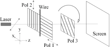
Figure 1 shows a typical setup for the quantum eraser [22]. When there are no polarizers, an interference pattern composed of dark and bright fringes can be observed on the screen because light passing on the left of the wire is combining, or “interfering,” with light passing on the right-hand side. In other words, we have no information about which path each photon went.
When polarizers 1 and 2, which are called “which-path markers”, are positioned right behind the wire as shown in Figure 1, the launched light polarized in 45◦ direction from the Laser is polarized in perpendicular (x-polarized and y-polarized) by these polarizers. Then the interference pattern on the screen is erased because “which-path makers” have made available the information about which path each photon went.
When polarizer 3 is inserted in front of the screen with the polarization angle +45◦ or −45◦ in addition to “which-path makers”, the interference pattern reappears because polarizer 3 has made the information of “which-path makers” unusable.
We can produce a mathematical description of the erasure and reappearance of the interference pattern as follows. Thex- andy-polarized photons passing through polarizers 1 and 2 can be expressed by the quantum-superposition states as follows.
|x= √1 2|++
1
√
2|− (5)
and
|y= √1 2|+ −
1
√
2|− (6)
where “+” and “−” represent polarizations +45◦ and−45◦ with respect tox.
The photons pass through polarizers 1 and 2 are polarized at right angles to each other as seen in the left-hand side of Eqs. (5) and (6), which prevent the interference pattern. In other words, “which-path makers” have made available the information about which “which-path each photon went. Although there are same polarized states in the right-hand side of Eqs. (5) and (6), the interference patterns consisting of bright and dark fringes made by +45◦ and −45◦ polarized states are reverted images and annihilate each other. Therefore, sum total of the images has no interference pattern.
When polarizer 3 is inserted with the polarization angle +45◦ or −45◦, only |+ or |−can pass through polarizer 3. Then the interference pattern made by either |+ or |−of both Eqs. (5) and (6) reappears, which means that we cannot identify which-path the photons had passed through, i.e., polarizer 3 has made the information of “which-path makers” unusable.
3. NEW EXPLANATION FOR QUANTUM ERASER
The mathematical description of the photon states passing through polarizers 1 and 2 used in the traditional explanation requires the quantum-superposition states in Eqs. (5) and (6), respectively.
the wave packet. These paradoxes are great problems not only with the traditional explanations but also for true nature of physics.
Although tensor form (covariant quantization) is a rigorous treatment as we will describe later, here we conveniently take advantage of the unobservable potentials that can eternally populate the whole space as waves independent of existence of the substantial photons. Therefore, we can replace the photon state |x with|x+|ζ, where|ζ is a state representing the unobservable potentials whose probability (or more like “interference”) amplitudes ζ|ζ= 0 in initial states as described in Eq. (4) (when there is no difference in phase and polarization angle as described below.). The unobservable potentials can be polarized by the polarizers because these potentials obey Maxwell equations and populate the whole space-time. Therefore, we should introduce the polarization terms with unobservable potentials.
Then the following states, which are identified as Eq. (4) introducing polarization terms similar to Eq. (3), can generate the same interference as the quantum-superposition states in Eqs. (5) and (6).
|x+|ζφ,x=|x+1 2γe
iφeiθ/2|x −1
2γe
−iφe−iθ/2|x
|y+|ζφ+1
2π,y=|y+
1 2γe
i(φ+12π)e−iθ/2|y −1
2γe
−i(φ+12π)eiθ/2|y
(7)
where γ2 =−1,φ and θ are the indefinite metric, the polarization angle of polarizer 3 measured from
x-axis and phase difference between left and right paths, respectively.
Therefore, when we observe only |x with polarizer 3, i.e., θ = 0, the intensity of the interference
I can be calculated as follows.
I∝(x|+ζφ,x|) (|x+|ζφ,x) =x|x−1
2x|x+ 1
2x|xcos(2φ+θ) = 1 2+
1
2cos(2φ+θ) = 1 2+
1
2cos(2φ) (8) Hence the output intensity by rotation angle of polarizer 3 is reproduced correctly.
When we observe|x and|y with polarizer 3, the intensity is obtained as follows.
I ∝
x|+ζφ,x|+y|+ζφ+1
2π,y| |x+|ζφ,x+|y+|ζφ+12π,y
(9) Because x|y=y|x= 0,
I ∝(x|+ζφ,x|) (|x+|ζφ,x) +
y|+ζφ+1
2π,y| |y+|ζφ+12π,y
(10) By using Eq. (8), we can obtain the following result.
I ∝ 1
2 + 1
2cos (2φ+θ) + 1 2 +
1
2cos (2φ+π−θ) = 1 + 1
2cos (2φ+θ)− 1
2cos (2φ−θ) (11) When φ = ±π, ±12π, I ∝ 1 and φ = ±14π, then I ∝ 1±sinθ, which reproduces the interference correctly.
In this new explanation, the polarization of substantial photons is fixed, and the photons cannot pass through the polarizer which has a different polarization angle. However, the unobservable potentials create the same interference as the superposition states of |+ and |− as described above. In the case of x-polarized single photon, the interference can be calculated by Eq. (7) replacing|y with |0. Then I ∝ 1 + 12cos(2φ+θ)− 12cos(2φ−θ) is obtained. Note that when we calculate the single photon interference by using photon number operator n1 = ˆA†1Aˆ1, we can obtain exact expression
I ∝ 12+12cos(2φ+θ) because0|0= 1=0|n1|0= 0, where ˆA1 is the photon annihilation operator
obtained from the vector potentials in Eq. (1) [14].
The above calculations are based on Schr¨odinger picture. We can obtain the same results based on Heisenberg picture. In Heisenberg picture, the photon number operator should be replaced by n = ( ˆA†1 + ˆA†p)( ˆA1 + ˆAp) [14], where ˆA1 and ˆAp (p : polarization = x, y, . . ., etc.) are the photon
annihilation operators obtained from the vector and scalar potentials in Eq. (1), respectively, which represent the substantial photons and modified operator introducing the polarization terms in Eq. (2), i.e., the polarized unobservable potentials, as follows.
ˆ
Ax= 1 2γe
iφeiθ/2Aˆ 1−
1 2γe
−iφe−iθ/2Aˆ
1, Aˆ†x =
1 2γe
−iφe−iθ/2Aˆ† 1−
1 2γe
iφeiθ/2Aˆ†
We can calculate Eq. (8) in Heisenberg picture as follows.
I=
n
ˆ
A†1+ ˆA†x Aˆ1+ ˆAxn =n|n1|n+n|Aˆ†xAˆx|n ∝1−
1 2+
1
2cos(2φ+θ) = 1 2+
1
2cos(2φ) (13) Note that the x-polarized photon annihilation operator should be represented by ˆA1+ ˆAx instead of
ˆ
A1 in Heisenberg picture [14]. When there are x- and y-polarized photons, the operator should be
represented by ( ˆA1+ ˆAx) + ( ˆA2+ ˆAy), where ˆA2 is a photon annihilation operator obtained from the
quantization of y-polarized vector potential, and ˆAy can be obtained by replacing φ withφ+ 12π and ˆ
A1, ˆA†1 with ˆA2, ˆA†2 in Eq. (12). Then we can calculate Eq. (9) in Heisenberg picture as follows.
I = n|( ˆA†1+ ˆA†x+ ˆA†2+ ˆA†y)( ˆA1+ ˆAx+ ˆA2+ ˆAy)|n
= n|n1|n+n|Aˆ†xAˆx|n+n|n2|n+n|Aˆ†yAˆy|n ∝1 +
1
2cos (2φ+θ)− 1
2cos (2φ−θ) (14) where we identify n|n1|n ≡ n|Aˆ†1Aˆ1|n = n|n2|n ≡ n|Aˆ†2Aˆ2|n = n assuming that there are the
same number (n) ofx- andy-polarized photons. Under the assumption|n ≡ |nx+|ny where|nx,|ny
are the x- and y-polarized n photon states, respectively, we can calculate ˆA1|n = ˆA1|nx+ ˆA1|ny =
√
n|n−1x and ˆA2|n = ˆA2|nx+ ˆA2|ny =√n|n−1y. In addition,n|Aˆ†1Aˆ2|n =n|Aˆ†2Aˆ1|n = 0 is
calculated.
The new explanation can describe that ˆAp or|0+|ζ which can be identified as vacuum, creates and annihilates the substantial photons through the interference.
Loosely speaking, the unobservable potentials are oriented by the polarizers such as Eq. (7) or Eq. (12). Then the substantial photons surf on the sea of the oriented potentials which can change into substantial photons through the interference.
Figure 1. Typical setup for the quantum eraser. Pol1 and Pol2 are fixed linear polarizers with polarizing axes perpendicular (xand y). Pol3 is a revolvable linear polarizer.
Figure 2. Typical setup for the delayed choice quantum eraser. QWP1 and QWP2 are quarter-wave plates aligned in front of the double slit with fast axes perpendicular. Pol1 is a linear polarizer. BBO (β−BaB2O4) crystal generates
entangled photons by spontaneous parametric down-conversion [23].
4. NEW EXPLANATION FOR DELAYED CHOICE QUANTUM ERASER
In this section, we show new explanation for Delayed Choice Quantum Eraser as shown in Figure 2 which consists of an entangled photon source and two detectors. The delayed choice has been demonstrated when the distance from BBO to polarizer 1 is longer than that from BBO to the double slit [23].
However, mathematical description for the phenomenon requires entangled state such as
|ψ= √1
2(|xs|yp+|ys|xp) (15) The entangled state declares that the state of the whole system is a quantum-superposition state consisting of |xs|yp and |ys|xp. Therefore, when the state of one photon (s or p) is observed and determined to be|x, that of the other photon (pors) suddenly changes from the quantum-superposition state into|yeven if the photons separate from each other, which postulates the existence of long-range correlation beyond the causality (spooky action at a distance). This postulate represents a critical defect and serious problem with the traditional explanations as pointed out in a paper by “Einstein, Podolsky and Rosen (EPR)” [2].
Hence we grapple with a strange physical phenomenon from the moment that we choose the polarization angle of polarizer 1 to the moment that BBO generates the entangle photon pairs.
The unobservable potentials, which can change from the potentials into substantial photons, eternally populate the whole space not forgetting the space between BBO and polarizer 1 independent of substantial photons. Hence, the space will be populated by the unobservable potentials which are oriented by polarizer 1 as described above. More precisely, the potentials determine the polarization of substantial photons in the space in advance depending on the polarization angle of polarizer 1.
For example, if we choose the polarization angle of polarizer 1 to φ which is measured from the polarization angle ψ of created photons, then the unobservable potential is oriented to |0 +|ζφ =
|0+ 12γei(φ−ψ)eiθ/2|0 − 12γe−i(φ−ψ)e−iθ/2|0 at polarizer 1 and propagates to BBO. BBO is forced to generate the photon pair with polarizationp: φand s: φ±12π according to the arrival potentials. The mathematical description is as follows. By applying a photon creation operator ˆAψ† to the polarized potentials, i.e.,
ˆ
Aψ†|0+ ˆAψ†|ζφ=|ψ+1 2γe
i(φ−ψ)eiθ/2|ψ −1
2γe
−i(φ−ψ)e−iθ/2|ψ (16)
Equation (16) can be calculated as the created photon state at BBO. Then the intensity of the created photon can be calculated in this setup (θ= 0) as follows.
I ∝ 1
2 + 1
2cos (2φ−2ψ) (17) In order to create a photon, i.e., I= 1,ψ=φwill be required.
Then the polarization of the photon pair is fixed by the unobservable potentials instead of the entangle state in Eq. (15). Therefore, when the polarization angle is set to the fast axis of QWP (Quarter-wave plate) 1 or 2, the interference pattern can be observed.
In this case, we are not aware of the determination of the polarization of the photon pair by the unobservable potentials. This is the reason that the state seems to be “entangled”, and the choice of the polarization angle of polarizer 1 seems to be “delayed”.
In order to confirm the new explanation, we should make experiments with a shutter between BBO and polarizer 1 as follows. First, close the shutter not to make a definite orientation of the unobservable potentials. After the entangled photon pairs are generated, open the shutter. When the photon s is detected by Ds, close the shutter again. After a time period, we excite BBO to generate the next entangled photon pairs. When the next pairs are generated, open the shutter again. By repeating these procedures, we can make a comparison between the traditional results and new result. If the definite orientation of the unobservable potentials as mentioned above is valid, no interference pattern can be observed even if the polarization angle of polarizer 1 is set to the fast axis of QWP 1 or 2 throughout the experiment.
Note that because the unobservable potentials obey Maxwell equations propagate at the speed of light, the above time period that prevents the unobservable potentials from being oriented should be longer than the distance between BBO and the shutter divided by the speed of light.
the long-range correlation beyond the causality as follows. From Eq. (7), the measurement results of photonssand p are expressed as follows.
Is ∝ 1
2 + 1
2cos(2φ), Ip ∝ 1 2−
1
2cos(2φ) (18) There is no such a classical correlation. The above results are identical to the traditional quantum-mechanical predictions and violate Bell’s inequalities. Therefore, the long-range correlation associated with the interference between the photons and unobservable potentials is observed in all the experimental setups presented here. This is the answer to the so called “setting-independence loophole” [24].
Therefore, the confirmation method for the preselected polarization case described above has to be carefully implemented. When there are no polarizers, the polarization is randomly selected. Hence, a detection frequency of photons byDp proportional to the intensity of measured photon will be extremely lower than the case when there are polarizers. The difference of the detection frequency will be the only way to distinguish the new explanation from traditional one.
5. TENSOR FORM OF THE ELECTROMAGNETIC FIELDS
We have introduced the operator by using γ2 =−1 such as Eq. (12), which expresses the unobservable potentials for convenience in calculation in the above. When we use tensor form of the electromagnetic fields, the operator and results can be spontaneously obtained in following manner. The following is almost the same as the description for the single photon interference in [14].
The electromagnetic potentials are expressed as following four-vector in Minkowski space.
Aμ=A0, A1, A2, A3= (φ/c,A) (19)
The four-current is also expressed as following four-vector.
jμ=j0, j1, j2, j3= (cρ,i) (20)
When we set the axes of Minkowski space tox0 =ct, x1 =x,x2 =y,x3 =z, Maxwell equations with Lorentz condition are expressed as follows.
Aμ=μ0jμ, ∂μAμ= 0 (21)
In addition, the conservation of charge divi + ∂ρ/∂t = 0 is expressed as ∂μjμ = 0, where
∂μ = (1/c∂t,1/∂x,1/∂y,1/∂z) = (1/∂x0,1/∂x1,1/∂x2,1/∂x3), and stands for the d’Alembertian:
≡∂μ∂μ≡∂2/c2∂t2−Δ.
The transformation between covariance and contravariance vectors can be calculated by using the simplest form of Minkowski metric tensor gμν as follows.
gμν =gμν =
⎡ ⎢ ⎣
1 0 0 0 0 −1 0 0 0 0 −1 0 0 0 0 −1
⎤ ⎥ ⎦
Aμ=gμνAν, Aμ=gμνAν
(22)
The following quadratic form of four-vectors is invariant under a Lorentz transformation.
(x0)2−(x1)2−(x2)2−(x3)2 (23) The above quadratic form applying a minus sign expresses the wave front equation and can be described by using metric tensor.
−gμνxμxν =−xμxμ=x2+y2+z2−c2t2 = 0 (24) This quadratic form which includes minus sign is also introduced to inner product of arbitrarily vectors and commutation relations in Minkowski space.
The four-vector potential satisfies Maxwell equations with vanishing four-vector current which can be expressed as following Fourier transform in terms of plane wave solutions [25].
Aμ(x) =
dk˜
3
λ=0
a(λ)(k) μ(λ)(k)e−ik·x+a(λ)†(k) μ(λ)∗(k)eik·x
˜
k = d
3k
2k0(2π)3
k0 =|k| (26)
where the unit vector of time-axis directionnand polarization vectors (μλ)(k) are introduced asn2= 1,
n0>0, and (0) =n, (1) and (2) are in the plane orthogonal tokand n (λ)(k)· (λ)(k) =−δ
λ,λ λ, λ = 1,2 (27)
(3) is in the plane (k, n) orthogonal to nand normalized
(3)(k)·n= 0,[ (3)(k)]2 =−1 (28)
Then (0) can be recognized as a polarization vector of scalar waves, (1) and (2) of transversal waves and (3) of a longitudinal wave. Then we take these vectors as the following easiest forms.
(0)= ⎛ ⎜ ⎝ 1 0 0 0 ⎞ ⎟
⎠ (1) = ⎛ ⎜ ⎝ 0 1 0 0 ⎞ ⎟
⎠ (2) = ⎛ ⎜ ⎝ 0 0 1 0 ⎞ ⎟
⎠ (3)= ⎛ ⎜ ⎝ 0 0 0 1 ⎞ ⎟ ⎠ (29)
When the Fourier coefficients of the four-vector potentials are replaced by operators as ˆAμ ≡ 3
λ=0aˆ(λ)(k) (λ)
μ (k), the commutation relations are obtained as follows.
ˆ
Aμ(k),Aˆ†ν(k)
=−gμνδ(k−k) (30) The time-axis component (corresponds to μ, ν = 0 scalar wave, i.e., scalar potential because (0)μ (k) = 0 (μ= 0)) has the opposite sign of the space axes. Because0|Aˆ0(k) ˆA†0(k)|0=−δ(k−k),
1|1=−0|0
d˜k|f(k)|2 (31)
where |1 = dkf˜ (k) ˆA†0(k)|0. Therefore, the time-axis component is the root cause of indefinite metric. Note that the products of the operators replaced from the four-vectors must introduce the same formalism.
ˆ
A†Aˆ=−gμνAˆμ†Aˆν (32)
In order to utilize the indefinite metric as follows, Coulomb gauge that removes the scalar potentials should not be used.
Here we can recognize the potentials before passing through polarizers 1 and 2 as
Aμ= (A0, A1, A2,0) (33)
where, we neglect the longitudinal wave which is considered to be unphysical presence, i.e., A3 = 0
for simplicity. When there are an x-polarized photon and scalar potential which pass through each polarizer, the potentials passing through the polarizers can be expressed as
A(xpol 1)μ=
1 2e
iθx/2A
(x)0, A(x)1,0,0
, A(xpol 2)μ=
1 2e
−iθx/2A
(x)0,0,0,0
(34) When these scalar potentials undergo a|φ|phase shift, i.e., the angle of polarizer 3, by passing through polarizer 3, the phase terms will be shifted to±i(|φ|+θx/2). Here we identify the number operators as
1|A†0A0|1 =1|A†1A1|1 =1|A†2A2|1= 1 because of the Lorentz invariance. Hence the single photon
interference in Eq. (8) or (18) is obtained as followings.
A(xpol 1,2→3)μ≡A(xpol 1→3)μ+A(xpol 2→3)μ =
cos
|φ|+θx 2
A(x)0, A(x)1,0,0
(35)
Is ∝ 1|A†(xpol 1,2→3)A(xpol 1,2→3)|1 =
1 2 −
1
Similarly, in the case of ay-polarized photon
A(ypol 1)μ =
1 2e
iθy/2A
(y)0,0,0,0
, A(ypol 2)μ=
1 2e
−iθy/2A
(y)0,0, A(y)2,0
(37)
A(ypol 1,2→3)μ ≡A(ypol 1→3)μ+A(ypol 2→3)μ=
cos
|φ|+θy 2
A(y)0,0, A(y)2,0
(38) Then
Ip ∝ 1|A†(ypol 1,2→3)A(ypol 1,2→3)|1=
1 2−
1
2cos(2|φ|+θy) (39) By choosingθ≡θx =−(θy+π), i.e., the potentials undergoπ phase shift and the relatively-same phase shift at polarizers 1 and 2 when being divided,
Is ∝ 1
2 − 1
2cos(2|φ|+θ), Ip ∝ 1 2 +
1
2cos(2|φ| −θ) (40) Hence, we should choose θ =θ+π to correct the reversed signs, which is attributed to the difference between usingγ2 =−1 and tensor form.
In case of both polarization photons exist, the potentials just before polarizer 3 will be expressed by summation of Eqs. (34) and (37). Then the potentials that undergo a |φ|phase shift by polarizer 3 can be expressed as follows.
A(x,ypol 1,2→3)μ=
A(x)0cos
|φ|+θx 2
+A(y)0cos
|φ|+θy 2
, A(x)1, A(y)2,0
(41) Therefore, the photon number operator of the output of polarizer 3 can be calculated as follows.
A†(x,ypol 1,2→3)A(x,ypol 1,2→3)
= −A†(x)0A(x)0cos2
|φ|+θx 2
−A†(y)0A(y)0cos2
|φ|+ θy 2
+A†(x)1A(x)1+A†(y)2A(y)2−(A†(x)0A(y)0+A†(y)0A(x)0) cos
|φ|+θx 2
cos
|φ|+θy 2
(42) Then by choosing θ≡θx =−(θy+π),
1|A†(x,ypol 1,2→3)A(x,ypol 1,2→3)|1 = 1− 1
2cos(2|φ|+θ) + 1
2cos(2|φ| −θ)
−1|(A†(x)0A(y)0+A†(y)0A(x)0)|1cos
|φ|+θ 2 sin |φ|−θ 2 (43) Here we should recognize |1= (|1x+|1y) as mentioned above, andA(x)0 and A(y)0 annihilatex and
y-polarized photon, respectively, i.e.,A(x)0|1=|0x and A(y)0|1=|0y. Becausex0|0y = 0,
−1
A†(x)0A(y)0+A(†y)0A(x)01 = 0 (44) Hence Eq. (43) corresponds to Eqs. (11) and (14) except theπ phase shift of θ.
6. DISCUSSION
In this paper, we have taken advantage of the indefinite metric property of scalar potentials. Here we discuss what the scalar field represents.
Usually in quantum optics, we can split the electric field and current density by using Coulomb gauge as follows [26].
E=ET+EL, ∇ ·ET= 0, ∇ ×EL= 0
i=iT+iL, ∇ ·iT = 0, ∇ ×iL= 0
where the indexes “T” and “L” stand for “Transverse” and “Longitudinal”, respectively. By using electromagnetic potentials, “Transverse”components of Maxwell equations can be described as follows.
∇ ×ET=− ∂B
∂t , ∇ ×B=
1
c2 ∂ET
∂t +μ0iT
ET=− ∂A
∂t , ∇ ·B= 0
(46)
whereB is the magnetic field. We can also obtain following “Longitudinal” components. EL=−∇φ, ∇ ·EL =
ρ
0
iL= 0∇ ∂φ
∂t =− 0 ∂EL
∂t
(47)
Hence the transverse component seems associated with the magnetic field variation, and the longitudinal component seems associated with charges as the regular scalar potential.
However, these associations are justified in a particular coordinate system, i.e., “relative associations”. When the coordinate system is changed according to Lorentz transformation, “Transverse” and “Longitudinal” components are mixed. Then the associations have no meaning which is the important assertion of relativity [27]. This is why we equate scalar potentials with vector potentials, i.e., identify the number operators as1|A†0A0|1=1|A1†A1|1 =1|A†2A2|1= 1 by Lorentz
invariance. In addition, the Coulomb gauge removes the explicit covariance of Maxwell equations. Hence we would better use Maxwell equations (21) with Lorentz gauge. By utilizing the linearity of Equation (21), we can express Maxwell equations with Lorentz condition as follows.
Aμ=
Aμ(mat)+Aμ(vac)
=μ0jμ ∂μAμ=∂μ
Aμ(mat)+Aμ(vac)
= 0
(48)
where index “mat” and “vac” mean “matter” associated with four-current and “vacuum”, respectively. If we naturally assume that there are no four-current in vacuum, then Aμ(mat) and Aμ(vac) obey the following Maxwell equations respectively.
Aμ(mat) = μ0jμ, ∂μAμ(mat)= 0 (49)
Aμ(vac) = 0, ∂μAμ(vac)= 0 (50)
Equation (49) will express substantial photon excited by the four-current. Note that when we consider the spatial domain far from and exclude the four-current, Equation (50) replacingAμ(vac) with
Aμ(mat) can express the motion of the potentials in the domain associated with the four-current.
In contrast, Equation (50) expresses the motion of the potentials unrelated to “matter” in vacuum. Therefore, we can imagine that vacuum is the sea filled with unobservable potentials, which evokes the concept of an ether. Although the static ether has been rejected by special relativity [27], the above filling potentials are not static entity but propagate at the speed of light. Aharonov-Bohm effect clearly presents that the unobservable potentials without electromagnetic field can cause electron interference [16, 28, 29]. By the same token, the filling potentials in Eq. (50) can cause interference with substantial photon, Eq. (49) as if it were a local oscillator for homodyne detection attached to space-time as discussed in [14].
We generally calculate photon related phenomena usingAμin Eq. (48) unconsciously, i.e., without separation into “matter” and “vacuum”. However, we cannot distinguishAμ(mat) from Aμ(vac), which is very much like distinguish sea spray from seawater. Indeed, no separation will be required because both are ever-changing potentials derived from the same Maxwell equation (48). Therefore, the filling potentials in vacuum can expel and incorporate the potentials associated with “matter”, which makes us imagine that vacuum can create and annihilate substantial photon.
The scalar field used in this paper correspond to the scalar component of this filling potentials in the literature.
7. CONCLUSIONS
We have presented that the quantum eraser can be explained without quantum-superposition states by introducing the unobservable (scalar) potentials whose probability (or more like “interference”) amplitudes are zero. The explanation presents the concept that vacuum can create and annihilate the substantial photons.
We have also investigated the delayed choice experiment under the assumption that the polarization of the photon pairs is determined by the unobservable (scalar) potentials which are oriented by the setup of the experiment in advance. Moreover, we show that the interference between the photons and unobservable potentials makes the long-range correlation beyond the causality that does not really exist in nature but seems to exist regardless of the assumption. In addition to these discussions based on a method for convenience in calculation, we have shown rigorous mathematical treatment using tensor form (covariant quantization).
The new explanations obtained in the present paper are more general and physically consistent than traditional explanations which require paradoxical quantum-superposition states and entangled states.
The other experiments and considerations have been reported, which seem like paradoxes [11– 13, 24, 30–32]. We believe that the paradoxes can be avoided by the new explanation. Moreover, we should investigate whether engineering applications based on wave packet reduction or entangled states are feasible technologies or not, because an inevitable conclusion by the rigorous derivation described in this paper can remove the paradoxical base concepts of the applications.
The new explanation presented here and [14] compel a restructuring of the traditional standard quantum theory. However, this is the real natural law without the enigmatic and paradoxical thought processes such as quantum-superposition and entanglement based on the “probabilistic interpretation”. ACKNOWLEDGMENT
The author would like to thank K. Sato and Dr. S. Takasaka for their helpful discussions. REFERENCES
1. Trimmer, J. D., “The present situation in quantum mechanics: A translation of Schr¨odinger’s “cat paradox” paper,”Proceedings of the American Philosophical Society, Vol. 124, 323–338, Oct. 1980. 2. Einstein, A., B. Podolsky, and N. Rosen, “Can quantum-mechanical description of physical reality
be considered complete?,” Phys. Rev., Vol. 47, 777–780, May 1935.
3. Bohm, D., “A suggested interpretation of the quantum theory in terms of “hidden” variables. I,” Phys. Rev., Vol. 85, 166–179, Jan. 1952.
4. Bohm, D., “A suggested interpretation of the quantum theory in terms of “hidden” variables. II,” Phys. Rev., Vol. 85, 180–193, Jan. 1952.
5. Bell, J. S., “On the problem of hidden variables in quantum mechanics,” Rev. Mod. Phys., Vol. 38, 447–452, Jul. 1966.
6. Oriols, X. and J. Mompart, “Overview of bohmian mechanics,”ArXiv e-prints, Jun. 2012.
7. Pylkk¨anen, P., B. J. Hiley, and I. P¨attiniemi, “Bohm’s approach and individuality,”ArXiv e-prints, May 2014.
8. Durr, D., S. Goldstein, T. Norsen, W. Struyve, and N. Zanghi, “Can Bohmian mechanics be made relativistic?,” Royal Society of London Proceedings Series A, Vol. 470, 30699, Dec. 2013.
9. Allori, V., S. Goldstein, R. Tumulka, and N. Zanghi, “Predictions and primitive ontology in quantum foundations: A study of examples,” ArXiv e-prints, May 2012.
10. Dennis, G., M. A. de Gosson, and B. J. Hiley, “Fermi’s ansatz and bohm’s quantum potential,” Physics Letters A, Vol. 378, No. 3233, 2363–2366, 2014.
12. Aspect, A., P. Grangier, and G. Roger, “Experimental realization of einstein-podolsky-rosen-bohm gedankenexperiment: A new violation of bell’s inequalities,”Physical Review Letters, Vol. 49, No. 2, 91–94, 1982.
13. Aspect, A., J. Dalibard, and G. Roger, “Experimental test of bell’s inequalities using time-varying analyzers,”Physical Review Letters, Vol. 49, No. 25, 1804, 1982.
14. Morimoto, M., “Unobservable potentials to explain single photon and electron interference,” Journal of Computational and Theoretical Nanoscience, Vol. 14, No. 8, 4121–4132, 2017.
15. Ehrenberg, W. and R. E. Siday, “The refractive index in electron optics and the principles of dynamics,”Proceedings of the Physical Society, Section B, Vol. 62, No. 1, 8, 1949.
16. Aharonov, Y. and D. Bohm, “Significance of electromagnetic potentials in the quantum theory,” Phys. Rev., Vol. 115, 485–491, Aug. 1959.
17. Meis, C., “Vector potential quantization and the quantum vacuum,” Physics Research International, Vol. 5, 2014.
18. Yang, C. N. and R. L. Mills, “Conservation of isotopic spin and isotopic gauge invariance,” Phys. Rev., Vol. 96, 191–195, Oct. 1954.
19. Wu, T. T. and C. N. Yang, “Concept of nonintegrable phase factors and global formulation of gauge fields,”Phys. Rev. D, Vol. 12, 3845–3857, Dec. 1975.
20. Weinberg, S., “A model of leptons,”Phys. Rev. Lett., Vol. 19, 1264–1266, Nov. 1967.
21. Utiyama, R., “Invariant theoretical interpretation of interaction,”Phys. Rev., Vol. 101, 1597–1607, Mar. 1956.
22. Rachel Hillmer, P. K., “A do-it-yourself quantum eraser,”Scientific American, No. 5, 9095, 2007. 23. Walborn, S. P., M. O. Terra Cunha, S. P’adua, and C. H. Monken, “Double-slit quantum eraser,”
Phys. Rev. A, Vol. 65, 033818, Feb. 2002.
24. Handsteiner, J., A. S. Friedman, D. Rauch, J. Gallicchio, B. Liu, H. Hosp, J. Kofler, D. Bricher, M. Fink, C. Leung, A. Mark, H. T. Nguyen, I. Sanders, F. Steinlechner, R. Ursin, S. Wengerowsky, A. H. Guth, D. I. Kaiser, T. Scheidl, and A. Zeilinger, “Cosmic bell test: Measurement settings from milky way stars,”Physical Review Letters, Vol. 118, 060401, Feb. 2017.
25. Itzykson, C. and J. B. Zuber,Quantum Field Theory, McGraw-Hill, 1985.
26. Loudon, R.,The Quantum Theory of Light, 2nd Edition, Oxford University Press, 1983.
27. Einstein, A., “Zur elektrodynamik bewegter krper,”Annalen der Physik, Vol. 322, No. 10, 891–921, 1905.
28. Tonomura, A., T. Matsuda, J. Endo, T. Arii, and K. Mihama, “Direct observation of fine structure of magnetic domain walls by electron holography,” Physical Review Letters, Vol. 44, 1430–1433, May 1980.
29. Tonomura, A., H. Umezaki, T. Matsuda, N. Osakabe, J. Endo, and Y. Sugita, “Is magnetic flux quantized in a toroidal ferromagnet?,” Physical Review Letters, Vol. 51, 331–334, Aug. 1983. 30. Salart, D., A. Baas, J. A. W. van Houwelingen, N. Gisin, and H. Zbinden, “Spacelike separation in
a bell test assuming gravitationally induced collapses,” Physical Review Letters, Vol. 100, 220404, Jun. 2008.
31. Kim, Y.-H., R. Yu, S. P. Kulik, Y. Shih, and M. O. Scully, “Delayed “choice” quantum eraser,” Physical Review Letters, Vol. 84, 1–5, Jan. 2000.