A Decomposition Method for Computing Radiowave Propagation
Loss Using Three-Dimensional Parabolic Equation
Guizhen Lu1, *, Ruidong Wang1, Zhi Cao2, and Kehua Jiang1
Abstract—The parabolic equation (PE) method is widely used in radiowave propagation predictions. It has the advantages of high efficiency and stability, but it will lead to greater predicting errors in some situations, because the effects of transverse terrain gradients are not modeled. This problem can be solved by extending the 2D PE to the three-dimensional (3D) PE. However, the computing efficiency will degrade because of large scale matrix operations. In this paper, a new method is presented, in which the 3D PE is decomposed into two 2D PEs. It increases the computational efficiency and accuracy effectively. To verify the capability of the proposed method in radiowave propagation prediction, an experiment platform was set up. The computational results using this new method are compared with the experimental and Method of Moment (MoM) numerical computational results. Good agreements are achieved in the comparison.
1. INTRODUCTION
The study of radiowave propagation under complex environments is vitally important for improving the effective signal coverage in wireless communication and television broadcasting with plenty of urban buildings as well as mountainous terrains. It presents a big challenge due to the multiple wave propagation mechanisms involving the line of sight, diffraction and scattering propagation and the characteristic of large scale computation. The major issues refer to how to keep the computational accuracy and conducting the large scale computation at the same time. To meet the request for large scale computation of actual engineering problems, the modified empirical formulas are often used for analysis and computation with the drawback of poor computational accuracy, and the variance of the predicted propagation loss is generally 2 to 5 dB for the flat terrain, but for the complex terrain, the variance of the predicted propagation loss is usually about 5 to 10 dB. Many computational methods have been developed to improve the predicted accuracy. The commonly used methods are geometric diffraction methods, path integration methods and FDTD. It is hard to meet the requirement of engineering computation because these methods are computationally expensive and require high data accuracy of the terrain database at the same time [1].
The Parabolic Equation (PE) method is a computational method for radiowave propagation loss besides the full wave method and ray tracing method, and has become a research focus. The PE method has high potential in radiowave propagation of mobile communication and broadcasting and television signal coverage as it can not only deal with complex terrain boundary conditions accurately, but also deal with complex atmosphere waveguide structure. Compared with the full wave method, the PE method deals with an unidirectional wave propagation, in which the equation can be solved by the step marching method in the propagation direction. The PE method can reduce the computational complexity of the full wave equation.
Received 20 September 2015, Accepted 16 November 2015, Scheduled 24 November 2015
* Corresponding author: Guizhen Lu ([email protected]).
1 School of Information Engineering Communication University of China, China. 2 Academy of Broadcasting Planning SARFT,
The PE method was firstly suggested in 1946 as Leontovich and Fock analyzed electromagnetic wave propagation problem in inhomogeneous atmosphere [2]. In 1977, Tappert solved PE by adopting Fourier split-step method in acoustics problem, showing that PE has the potential of solving large scale propagation problems [3]. Kuttler and Dockery applied the Fourier split-step method in analyzing radiowave propagation problems in the troposphere atmospheric waveguide [4]. Dockery and Kuttler introduced hybrid Fourier split-step method to analyze the impedance boundary condition propagation problems in 1996 [5]. In 1997, Levy adopted the Finite Difference (FD) method to solve PE in the irregular terrain radiowave propagation problem [6].
Normally, FD is used in middle scale computational problems while the Fourier split-step method can be applied in large scale computational problems. The advantage of FD is that it can simulate complex terrain boundary conditions, and its disadvantage is that its computational efficiency is lower than the Fourier split-step method. The Fourier split-step method has the advantage of good numerical computation stability and high computational efficiency. Ozgun introduced the recursive two-way PE method dealing with backward scattering of complex terrains as the Fourier split-step method was a forward marching method and could not deal with the backward scattering of complex terrains [7].
As the initial value of the PE has a big effect on the computational results, Apaydm and Sevgi studied how to determine the initial value of the PE [8]. The application of PE in horizontally inhomogeneous environments was studied by Barrios [9]. Hitney combined the ray-tracing and parabolic equation techniques to obtain fast solutions of very large scale radiowave propagation problems [10]. However, the above mentioned methods used two-dimension (2D) PE for solving tree-dimension (3D) problems, which can only be applied to axially symmetric 3D problems. The 2D PE only considers the irregularities in the vertical direction of complex terrains and ignores the irregularities in the horizontal direction. It cannot deal with horizontal terrain irregularities if they exist. To break through the limits of using 2D PE for the horizontal irregular terrains, Zelley built a model based on the implicit finite difference method to solve 3D PE [11]. Although the computing progress of the implicit finite difference method for wave propagation problems with various terrains is simpler than other methods because it can deal with the terrain boundary conditions more flexibly, it needs matrix operations with intensive computation and requires large computer memories. Saini and Casiraghi studied the 3D split-step Flourier transformation method, in which a 2D plane Flourier transformation was used, and the plane was perpendicular to the propagation direction [12]. Compared with the 3D finite difference method, 3D split-step Flourier transformation method decreased the degree of computation complexity, but the computational amount was still very large for large scale computing problems. Iqbal and Jeoti used wavelet transforming method to substitute Flourier transforming method to solve PE, and it was found that wavelet transforming method can improve calculation efficiency [13]. To overcome the difficulty that PE can only calculate unidirectional wave propagation problems, Ozgun proposed a technique for solving the PE in the two-way propagation using the iterative technique [14]. Apaydin and Ozgun solved complex terrain wave propagation problems using Finite Element Method (FEM) based on 2D PE [15]. The advantage of this solution is that it can process complex terrain boundary conditions, and the disadvantage is that it requires large computing memories and time.
Considering the request for improving prediction accuracy of large scale radiowave propagation, a new method is proposed in the paper, in which a 3D problem is decomposed into two 2D problems. The presented method can decrease the computation complexity compared with 3D PE. The basic idea of the proposed method is an assumption that the diffraction wave is attributed to the shortest-path diffraction, so that solving the 3D PE can be simplified to solving two 2D PE problems, and the calculation amount is decreased. Compared with the existing methods, this new method can process the wave propagation problem over the horizontally irregularity terrain with the same computation complexity as 2D PE.
2. THEORY ANALYSIS
propagation. When the PE was applied in complex-terrain radiowave propagation, the transverse change of complex terrains cannot be analyzed using 2D PE, and the computation complexity of 3D PE is large than 2D PE. The ray tracing methods can be applied in the prediction of radiowave propagation at high frequencies. By the ray tracing method, it is needed to find out the straight ray and diffraction ray, which contribute most to the receive signal as these rays have the shortest propagation path. Similarly, in order to solve the 3D PE, the main consideration is given to the straight wave and diffraction wave with the shortest propagation path, which can largely decrease the computational complexity of PE. The theoretical analysis is conducted based on the above considerations. Firstly, we started from the 3D Helmholtz equation. It is written as
∂2ψ
∂x2 +
∂2ψ
∂y2 +
∂2ψ
∂z2 +k
2ψ= 0 (1)
The wave function in Equation (1) can be replaced with the following expression
ψ(x, y, z) =u(x, y, z)·exp(ikx) (2)
Then, the equation about the reduced functionu(x, y, z) is
∂2u
∂x2 + 2ik
∂u
∂x +
∂2u
∂y2 +
∂2u
∂z2 = 0 (3)
By using the operator decomposition formula
∂
∂x+ik(1−Q)
·
∂
∂x +ik(1 +Q)
= 0 (4)
Q=
1− 1
k2 ·
∂2
∂y2 −
1
k2 ·
∂2
∂z2 (5)
the 3D PE is obtained as [11]:
∂u
∂x+
i
2k ·
∂2u
∂y2 +
i
2k ·
∂2u
∂z2 = 0 (6)
It is assumed that the 3D functionu(x, y, z) can be expressed as the sum of two 2D functions
u(x, y, z)≈u1(x, y) +u2(x, z) (7)
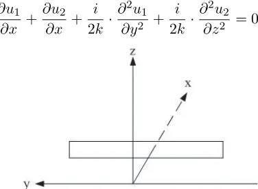
Similar to the geometrical diffraction theory, the main contributions to the receiving point come from vertical plane diffraction and horizontal plane diffraction, in which the diffraction waves have the shortest propagation path. Each plane diffraction is a 2D problem, and the 3D wave propagation problem can be approximated with two 2D wave problems superposition. Fig. 1 depicts the diffraction problem of 3D space.
The functionu2(x, z) in formula (7) is propagation waves in (x, z) plane and can be solved using 2D PE. The functionu1(x, y) in formula (7) is propagation waves in the (x, y) plane in Fig. 1. For the waves not in these two planes, they has little contribution to the received signal. By applying Equation (7), Equation (6) can be rewritten as
∂u1
∂x +
∂u2
∂x +
i
2k ·
∂2u
1
∂y2 +
i
2k·
∂2u
2
∂z2 = 0 (8)
Equation (8) can be further reduced to two 2D PE problems
∂u1
∂x +
i
2k ·
∂2u
1
∂y2 = 0 (9)
∂u2
∂x +
i
2k ·
∂2u
2
∂z2 = 0 (10)
Equations (9) and (10) can be solved by split-step Fourier transformation method, and the split-step Fourier transformation formulas for 3D space problems are obtained
u1(x+δx, y) = F−1
F
exp
−ip21·δx 2k
·u1(x, y)
(11)
u2(x+δx, z) = F−1
F
exp
−ip22·δx 2k
·u2(x, z)
(12)
In formulas (11) and (12),p1is thepspace variable after Fourier transformation againstyvariable,
p2 the p space variable after Fourier transformation against z variable, x the propagation directional space variable, and δx the step size of x direction. After computingu1(x, y) and u2(x, z), respectively, using formula (7), the receiving position signal can be obtained. To compare with experimental results, the received signal amplitude is transformed into propagation loss and the formulas are:
P L(dB) = −20·log10(|u|) + 20·log10(4π) + 20·log10(x)−20·log10(λ) (13)
E(dBV/m) = P t(dBW)−P L(dB) (14)
wherePt is the transmitted power,E the field strength andx the propagation distance variable.
3. COMPUTATION AND EXPERIMENT RESULTS
Multiple knife edge obstacle diffraction is a typically complex environment electromagnetic wave propagation problem. Many practical electromagnetic wave propagation prediction formulas are modified based on single knife edge diffraction. So the knife edge diffraction problem is chosen to verify the aforementioned method. In order to verify the proposed method, we compared its results with the experiment measurement and moment method calculation results. The experimental measurements were conducted in an indoor experimental environment to study knife edge radiowave diffraction problems. The experimental platform was constructed on a perfectly conductive plate and surrounded by absorbing materials. The working signal frequency was chosen at 9.35 GHz. The transmitting antenna was a monopole antenna, and the receiving antenna was a wave-guide probe. In the single knife edge diffraction experiment, to compare with 2D PE computing results, a 6.5 cm high metal strip was used as knife edge obstacle, and the width of the strip metal was long enough to avoid side diffraction. Fig. 2 shows the experimental results and 2D PE computing results about the single knife edge diffraction. It can be seen that the experimental results are consistent with PE calculation ones.
0 0.5 1 1.5 2 2.5 -100
-90 -80 -70 -60 -50 -40 -30 -20 -10 0
Distance (m)
Propagation Loss (dB)
PE Exp
Figure 2. Comparative results of the 2D PE computation and experiments for the single knife edge. The height of the obstacle is 6.5 cm and the width is 30 cm.
0 0.5 1 1.5 2
40 50 60 70 80 90 100 110 120 130
Distance (m)
Field (dBv/m)
PE MoM
Figure 3. Comparative results of decomposition 3D PE and MoM computation for the 3D single knife edge. The height of obstacle is 6.5 cm and the width is 10 cm.
Figure 4. The canonical 3D geometry of double finite-size knife edges.
0 0.5 1 1.5 2
50 60 70 80 90 100 110 120 130
Distance (m)
Field (dBv/m)
PE MoM
Figure 5. Comparative results of decomposition 3D PE and MoM computation for 3D double knife edges. The height of obstacle is 6.5 cm and the width is 10 cm.
0 200 400 600 800 1000 1200 1400 1600
10-5 10-4 10-3 10-2 10-1
Number of Variables
Computing Time(s)
1DFFT 2DFFF
method, we considered double knife edge diffraction problem, which is depicted in Fig. 4. To illustrate the horizontal situated position of the obstacles, Fig. 4 shows the pattern of transverse direction. The distance between the two obstacles is 0.3 m, and the obstacles are perpendicular to the propagation direction. Fig. 5 shows the comparative results of decomposition 3D PE and MoM computation for finite width double knife edge obstacles. The curves show the results of the field strength between the two obstacles. MoM computation presents fluctuant results, but decomposition 3D PE does not. The difference is because PE only deals with the forward propagation wave, and the signal fluctuation caused by forward propagation and backward propagation interference is not modeled in the range of two obstacles.
4. INVESTIGATIONS OF THE COMPUTATIONAL TIME AND THE COMPLEXITY
The presented method can improve the SSFT computing efficiency, which is very important in the large scale engineering wave propagation problems. In 3D SSFT, at each step along the range, a 2D FFT and IFFT transform is performed with the computational complexity ofO(N∗M∗(log(N) + log(M)), whereN is the size inydirection and M the size inz direction. In the presented method of this paper, the time complexity isO(N∗log(N) +M∗log(M)) at each step along the range. The compared results of computational complexity for these two algorithms are shown in Fig. 6. The curve with ‘∗’ represents the results of the algorithm presented in this paper, in which two 1D FFTs are required at each iteration step; the curve with ‘o’ represents the results of the 3-D SSFT algorithm, in which the 2D SSFT is required. The two smooth curves show the theoretical results of the 2D FFT and 1D FFT, respectively. In the simulation, the parameter M was taken as a fixed value 512, and N was changed from 16 to 1600. The computer CPU was the Intel(R) duo cpu E8400 @3.00 GHz. The average computing time at each step was 3.04e-2 s for 3D SSFT and 1.5795e-4 s for the new method. Their ratio was about 192. It can be seen that the presented method can improve the computing efficiency greatly.
5. CONCLUSIONS
This paper discusses the 3D PE computational method for the radiowave propagation problems in complex environments. Radiowave propagation in wireless communication and radio and TV broadcasting is a large scale computing problem, and it has a special requirement for the computational memory and speed. Traditional empirical formulae have the advantage of low degree of computational complexity, but their computational accuracy is very low. If we adopt the wave equation to solve electromagnetic propagation problems in 3D space, although it can meet the accuracy requirement, the amount of computation is very large. The currently used 2D PE method can only deal with the irregularities in the vertical direction and cannot deal with the horizontal irregularities of terrains. In this paper, we started with the wave equation and proposed a new method using two 2D PEs to solve the 3D PE. Through the comparison with indoor experimental results and MoM computational results, the feasibility of the proposed method was verified. This method satisfies the requests of computing accuracy and large scale computation. It expands the application scope of fast computation and can model the horizontal irregularities of terrains at the same time.
REFERENCES
1. Recmmendation ITU-R P.1546-2, “Method for point to area prediction for terratrial services in the frequency range 30 MHz to 3000 MHz,” International Telecommunication Union Geneva, 2005. 2. Leontovich, M. A. and V. A. Fock, “Solution of propagation of electromagnetic waves along the
Earths surface by the method of parabolic equations,” J. Phys. USSR, Vol. 10, 13–23, 1946. 3. Tappert, F., “The parabolic equation method,”Wave Propagation in Underwater Acoustics, J. B.
Keller and J. S. Papadakis (eds.), 224–287, Springer-Verlag, New York, 1977.
5. Dockery, G. D. and J. R. Kuttler, “An improved impedance-boundary algorithm for Fourier split-step solution of parabolic wave equation,” IEEE Trans. AP, Vol. 44, No. 12, 1592–1599, 1996. 6. Levy, M. F., “Transparent boundary conditions for parabolic equation solutions of radiowave
propagation problems,” IEEE Trans. AP, Vol. 45, No. 9, 66–72, 1997.
7. Ozgun, O., “Two-way Fourier split step algorithm over variable terrain with narrow and wide angle propagators,” Antennas and Propagation Society International Symposium 2010 IEEE, 2010. 8. Apaydm, G. and L. Sevgi, “Groundwave propagation at short ranges and accurate source
modeling,”IEEE Mag. AP, Vol. 55, No. 3, 245–262, 2013.
9. Barrios, A. E., “Parabolic equation modeling in horizontally inhomogeneous environments,” IEEE Trans. AP, Vol. 40, No. 7, 791–797, July 1992.
10. Hitney, H. V., “Hibrid ray optics and parabolic equation methods for radar propagation modeling,”
Proceeding of Radar 92, IEE Conf. Pub., No. 365, 58–61, 1992.
11. Zelley, C. A., “Radiowave propagation over irregular terrain using the 3D parabolic eaquation,”
IEEE Trans. AP, Vol. 47, No. 10, 1586–1596, 1999.
12. Saini, L. and U. Casiragh, “A 3D Fourier split-step technique for modelling microwave propagation in urban areas,” Proc. 4th Eur. Conf. Radio Relay Syst., 210–214, October 1993.
13. Iqbal, A. and V. Jeoti, “A split step wavelet method for radiowave propagation modelling in tropospheric ducts,” Radioengineering, Vol. 23, No. 4, 987–996, 2014.
14. Ozgun, O., “Recursive two-way parabolic equation approach for modeling terrain effects in tropospheric propagation,” IEEE Trans. AP, Vol. 57, No. 9, 2706–2714, 2009.