A Comparative Study for Breast Cancer Detection by Neural Approach for Different Configurations of the Microwave Imaging System

(1)

A Comparative Study for Breast Cancer Detection by Neural

Approach for Diﬀerent Conﬁgurations of the Microwave

Imaging System

Wassila Sekkal1, *, Lotfi Merad2, and Sidi M. Meriah1

Abstract—The study done in this paper focuses on the detection of breast cancer by neuronal approach, by rotating the transmitting antenna from 15◦, 30◦, 45◦, 60◦, 75◦, to 90◦ relative to its initial position which is of 0◦ (i.e., to the opposite of the receiving antenna). We have generated our database by using a CST electromagnetic simulator for each antenna location. Then the learning and test phases of our artiﬁcial neural network (ANN) are done for seven antennae locations using two learning algorithms which are: the Scaled Conjugate Gradient Back-propagation (Trainscg) and the Gradient Descent with Momentum (Traingdm). A comparative study was conducted for all the seven cases. The results obtained are very satisfying and show that the best location of the transmitter antenna is at 60◦ and that the learning algorithm Trainscg gives better results than Traingdm.

1. INTRODUCTION

Breast cancer is one of the most common cancers for women. For this, detection and early intervention are one of the most important factors in improving survival rates and quality of life of people with this type of cancer, since this is the time when treatment is most effective [1]. X-ray mammography is one of the most widely used imaging methods for early detection of breast cancer. However, despite significant progress in the improvement of the mammographic technique, persistent limitations lead to high rates of false negatives [2] and high rates of false positives [3] particularly in premenopausal women where increased breast density can obscure non-palpable lesions [4]. These false-positive diagnoses result in unnecessary biopsies, causing considerable distress to the patient and unnecessary financial burden on the health service. These limitations motivate the need of other methods that can overcome such limitations in a cost-effective manner.

Microwave imaging is considered as one of the most promising approaches for the detection of breast cancer during recent years. Several works have been conducted using a numerical breast model [3, 5– 7]. Microwave imaging consists of transmitting UWB signals through breast tissues and collecting received signals from different locations. When the breast is exposed to microwave radiation, the high water content of malignant breast tissues causes a more significant diffusion than healthy mammary tissues which have low water content [8]. It is reported, in the literature, that the increase in dielectric permittivity and conductivity for cancerous mammary tissues is three or more times greater than healthy tissues [5].

In this study, neural network in microwave imaging is going to be used in order to detect the presence of an eventual tumor in the breast. The proposed method has already been used in several studies [7–11]. However, the conﬁguration of the microwave system used only one position of the transmitting antenna

Received 19 November 2017, Accepted 14 February 2018, Scheduled 1 March 2018 * Corresponding author: Wassila Sekkal ([email protected]).

1 _{Laboratory of Telecommunications Tlemcen LTT, Faculty of Technology, University of Tlemcen, Algeria.}2_{2nd Cycle Department,}

(2)

network using the two algorithms. Section 3 presents the obtained results. Finally, a conclusion is given to summarize the work done in this project and also provides new perspectives for future work.

2. PROPOSED METHOD

2.1. Breast Model

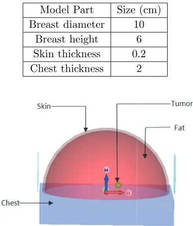
In this article, the model given in [5] is taken, which has a hemispherical shape, and our study is adapted to it, as presented in Table 1 and Fig. 1.

Table 1. Model dimensions.

Model Part Size (cm) Breast diameter 10

Breast height 6 Skin thickness 0.2 Chest thickness 2

Figure 1. Breast Model with tumor under CST.

The size of the tumor has been studied several times in the literature [6, 14]. A tumor of 0.25 cm in radius is taken with the following dielectric properties as shown in Table 2, whereσ is the conductivity in (Siemens/meter), andε_r is the relative permittivity [7].

2.2. Positioning of the Antenna and Creation of Data Base

(3)

Figure 2. Diﬀerent locations of the transmitting antenna.

To generate our seven databases, we proceed as follows as presented in [5]:

1) Place a pair of transmitter-receiver at opposite sides of the breast model; 2) Place a tumor at any location in the model;

3) Transmit a Gaussian pulse of a plane wave in the direction of theX andY axes; 4) Receive the signal on the opposite side;

5) Change the tumor location and repeat steps 3 and 4.

This process of data generation has been performed for 441 diﬀerent tumor locations along the X and Y axes for each position of the transmitter antenna. From this set two groups of received signals were formed as follows:

Group (1): A set of 341 signals were used for the learning of our ANN.

Group (2): A set of 100 signals were used for the testing phase of our ANN.

Table 2. Dielectric properties of the model.

Conductivityσ (S/m) Permittivity ε_r

Skin 1.49 37.9

Fat 0.14 5.14

Chest 1.85 53.5

Tumor 1.20 50

Output 2Hidden

input

Nodes _Node

layer layers layer

Output 3Hidden

input

layer layers layer

(a) (b)

(4)

samples obtained after interpolation with a step of 0.01 for each antenna location. The synthetic scheme of our model is illustrated in Fig. 4.

ANN MODEL P(Xi)

X

Y

The Position of The Tumor

Figure 4. Representation of the ANN model synthesis.

Table 3. The number of neurons in the input layer.

Location of antenna Time Segment Number of neurons in the input layer Antenna at 0◦ 2.8207 : 0.01 : 3.5937 78 Antenna at 15◦ 2.9431 : 0.01 : 3.5309 59 Antenna at 30◦ 2.5526 : 0.01 : 3.4988 95 Antenna at 45◦ 2.2019 : 0.01 : 3.5537 136 Antenna at 60◦ 2.4322 : 0.01 : 3.3203 89 Antenna at 75◦ 2.3777 : 0.01 : 3.0611 69 Antenna at 90◦ 2.4264 : 0.01 : 3.5911 117

Table 4 summarizes learning parameters of each neural network under MATLAB. The activation function used is a sigmoid function which has an output interval between [−1; 1]. Two learning algorithms are used: Scaled conjugate gradient backpropagation (Trainscg) and Gradient descent with momentum (Traingdm).

3. RESULTS

Once the learning phase was completed, the performance of our ANN was tested using group 2, shown in Figs. 5–11. In Tables 6–9 only 11 examples from group 2 are presented.

Tables 5 and 6 show the tumor detection results using the Scaled Conjugate Gradient (SCG) learning algorithm. The learning phase lasted respectively 10 hours, 3 minutes, 9 hours, 11 minutes, 2 hours, 5 hours, 5 hours for each antenna location.

Tables 7 and 8 show tumor detection results using the Gradient Descent With Momentum (GDM) learning algorithm. The learning phase lasted respectively 9 hours, 4 hours, 10 hours, 5 hours, 10 hours, 8 hours and 10 hours for each antenna location.

(5)

Table 4. The ANN parameters for transmitter antenna at 0◦, 15◦, 30◦, 45◦, 60◦, 75◦ and 90◦.

ANN Parameters Antenna Positions (◦)

0 15 30 45 60 75 90

Number of nodes in input layer 78 59 95 136 89 69 117

Number of nodes in hidden layer 1 45 45 45 45 45 45 45

Number of nodes in hidden layer 2 10 10 10 10 10 10 10

Number of nodes in hidden layer 3 - 5 - - - 5 5

Number of nodes in output layer 02 02 02 02 02 02 02

Activation function tansig tansig tansig tansig tansig tansig tansig

The learning Algorithm trainscg/traingdm

Table 5. Position of the tumor and the output of the ANN for a transmitter antenna at 0◦, 15◦, 30◦ and 45◦.

Real position of the tumor (cm/10)

Output of the ANN (SCG)

Antenna at 0◦ _{Antenna at 15}◦ _{Antenna at 30}◦ _{Antenna at 45}◦

X Y X Y X Y X Y X Y

0 0.9 0.000 0.9216 0.0024 0.9971 0.0005 0.8900 0.0000 0.90711

0.05 0.6 0.0482 0.6181 0.0422 0.6215 0.0439 0.6042 0.6715 6.2058

0.1 0.65 0.0103 0.6407 0.0987 0.6495 0.1048 0.6482 0.1224 0.6544

0.15 0.85 0.2097 0.8576 0.1362 0.9069 0.0013 0.8548 0.1903 0.8526

0.25 0.7 0.2437 0.6946 0.2532 0.6973 0.2508 0.6991 0.2519 0.6994

0.25 1 0.2483 0.9999 0.2624 0.9992 0.2476 0.9999 0.2257 0.9999

0.45 0.5 0.4449 0.5224 0.4578 0.4970 0.4500 0.4998 0.4504 0.5004

0.65 1 0.6513 1 0.6421 0.9997 0.6478 0.9999 0.6491 0.9999

0.8 0.65 0.8011 0.6452 0.7965 0.6335 0.7986 0.6493 0.8033 0.6504

0.9 0.8 0.8983 0.8017 0.8878 0.8067 0.8962 0.9997 0.8932 0.7982

0.95 1 0.9477 0.9972 0.9410 0.9998 0.9838 0.9997 0.9391 0.9997

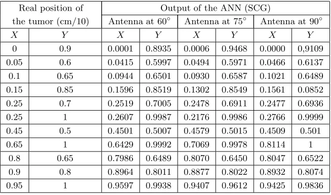
Table 6. Position of the tumor and the output of the ANN for a transmitter antenna at 60◦, 75◦ and 90◦.

Output of the ANN (SCG)

Antenna at 60◦ _{Antenna at 75}◦ _{Antenna at 90}◦

X Y X Y X Y X Y

0 0.9 0.0001 0.8935 0.0006 0.9468 0.0000 0,9109

0.05 0.6 0.0415 0.5997 0.0494 0.5971 0.0466 0.6137

0.1 0.65 0.0944 0.6501 0.0930 0.6587 0.1021 0.6489

0.15 0.85 0.1596 0.8519 0.1302 0.8549 0.1561 0.0852

0.25 0.7 0.2519 0.7005 0.2478 0.6911 0.2477 0.6936

0.25 1 0.2607 0.9987 0.2176 0.9986 0.2766 0.9999

0.45 0.5 0.4501 0.5007 0.4579 0.5015 0.4509 0.501

0.65 1 0.6429 0.9992 0.7069 0.9978 0.8114 1

0.8 0.65 0.7986 0.6489 0.8070 0.6450 0.8047 0.6522

0.9 0.8 0.8964 0.8011 0.8877 0.8022 0.8932 0.8074

(6)

0.25 1 0.2688 0.9693 0.2895 0.8915 0.2408 0.9943 0.2870 0,9919

0.45 0.5 0.4102 4.9518 0.4452 0.5002 0.4425 0.4980 0.4459 0.5015

0.65 1 0.6561 0.9758 0.6262 0.9194 0.6410 0.9990 0.6518 0.9909

0.8 0.65 0.7969 0.6298 0.8487 0.6752 0.7997 0.6514 0.7926 0.6487

0.9 0.8 0.9034 0.7989 0.8838 0.7656 0.9203 0.8053 0.9028 0.8010

0.95 1 0.9360 0.9757 0.9044 0.9296 0.9462 0.9919 0.9478 0.9836

Table 8. Position of the tumor and the output of the ANN for a transmitter antenna at 60◦, 75◦ and 90◦.

Output of the ANN (GDM)

Antenna at 60◦ Antenna at 75◦ Antenna at 90◦

X Y X Y X Y X Y

0 0.9 0.0234 0.8975 0.0487 0.9248 0.0008 0.8972 0.05 0.6 0.0537 0.6087 0.0789 0.5858 0.0495 0.6057 0.1 0.65 0.0902 0.6403 0.0918 0.6361 0.1042 0.6556 0.15 0.85 0.1320 0.8741 0.1357 0.8649 0.1510 0.8569 0.25 0.7 0.2555 0.7017 0.2254 0.7289 0.2444 0.6923 0.25 1 0.2510 0.9685 0.2245 0.2245 0.2458 0.9974 0.45 0.5 0.4558 0.5103 0.4517 0.4972 0.4491 0.5035 0.65 1 0.6304 0.9590 0.6709 0.9293 0.6617 0.9917 0.8 0.65 0.8021 0.6238 0.8546 0.7280 0.7894 0.6588 0.9 0.8 0.9043 0.8142 0.8912 0.8158 0.9216 0.8048 0.95 1 0.9234 0.9586 0.8305 0.8728 0.9379 0.9742

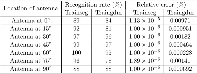
Table 9. Recognition rate and relative error for each antenna.

(7)

4. DISCUSSIONS

The detection of the tumor by a neural network have been studied for several locations of the transmitter antenna from 0◦ to 90◦ with a step of 15◦ (Fig. 2). Two algorithms have been used for the learning of each neural network trainscg and traingdm (see Tables 5–8). The positions obtained at the output of the ANN for each antenna location are very close to the real position under CST except for some of them that are relatively far as shown in Tables 5–8.

From Table 9, it is noted that for an antenna placed at 60◦ (Fig. 2) the best recognition rate is obtained with trainscg which is 100%, whereas the antenna locations obtained are, respectively, at 45◦ giving a rate of 99%, at 30◦ with a rate of 97%, at 75◦ with a rate of 96%, at 15◦ with a rate of 92%, at 0◦ with a rate of 89%, and ﬁnally a rate of 88% is noted for the antenna placed at 90◦ (Fig. 2).

The fact of making a rotation of the emitting antenna (Fig. 2) throughout the breast ensures a higher detection rate because with a single antenna position (antenna at 0◦) case studied in [16] there is a great risk that the tumor is not placed in the radiation ﬁeld of the transmitting antenna at this emplacement, and therefore, there will be no detection. It is also noticed that the learning algorithm trainscg gives a better result than traingdm.

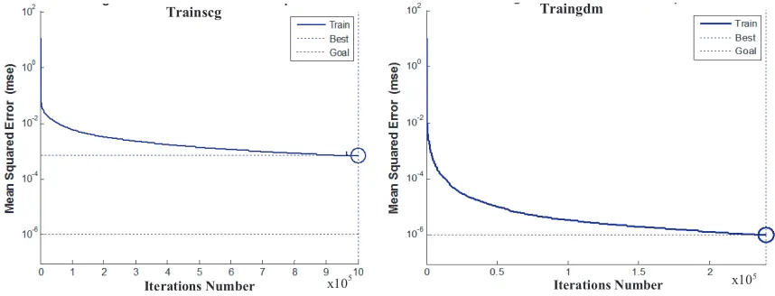
Trainscg Traingdm

Iterations Number x105 Iterations Number x105

Figure 5. Performance of the learning phase for trainscg and traingdm for an antenna at 0◦.

Traingdm Trainscg

(8)

Iterations Number

Iterations Number x10 x105

5

Iterations Number x10 4

Iterations Number x105

Iterations Number Iterations Number x105

(9)

Traingdm

Trainscg

5. CONCLUSIONS

In this work, a comparative study is conducted for the detection of breast cancer by an artiﬁcial neural network using two learning algorithms trainscg and traingdm. This is done by rotating the transmitter antenna on diﬀerent locations from 0◦ to 90◦ with step of 15◦. The learning algorithm trainscg gives better results than traingdm for the detection of tumor for each antenna location. These simulation results are very satisfactory in terms of detection.

This method gives an optimal recognition rate for diﬀerent locations of the transmitting antenna around the breast (60◦, 45◦, 30◦, 75◦) as shown in Table 9. So it is appreciated that it is a promising technique for detection of the tumor at any location in the breast. As perspectives, it is suggested to treat a similar study by decreasing the rotation step of the transmitting antenna. Also, it is interesting to look for a detection and localization of a tumor object in 3D. Finally, a study of a heterogeneous breast prototype is recommended.

REFERENCES

(10)

7. Chaudhary, S. S., R. K. Mishra, A. Swarup, and J. M. Thomas, “Dielectric properties of normal and malignant human breast tissues at radiowave and microwave frequencies,” Indian Journal of

Biochemistry and Biophysics, Vol. 21, 76–79, 1981.

8. Alshehri, S. A., “Experimental breast tumor detection using NN-based UWB imaging,” Progress

In Electromagnetics Research, Vol. 111, 447–465, 2011.

9. Alshehri, S. A., “3D experimental detection and discrimination of malignant and benign breast tumor using NN-based UWB imaging,”Progress In Electromagnetics Research, Vol. 116, 221–237, 2011.

10. O’Halloran, M., B. McGinley, R. C. Conceicao, F. Morgan, E. Jones, and M. Glavin, “Spiking neural networks for breast cancer classiﬁcation in a dielectrically heterogeneous breast,” Progress

In Electromagnetics Research, Vol. 113, 413–428, 2011.

11. Furundzicn, D., M. Djordjevic, and A. J. Bekic, “Neural networks approach to early breast cancer detection,”Journal of Systems Architecture, Vol. 44, No. 617, 6339, 1998.

12. Bindu, G., A. Lonappan, V. Thomas, C. K. Aanandan, and K. T. Mathew, “Active microwave imaging for breast cancer detection,” Progress In Electromagnetics Research, Vol. 58, 149–169, 2006.

13. Seladji, N., F. Z. Marouf, L. Merad, S. M. Meriah, F. T. Bendimerad, M. Bousahla, and N. Benahmed, “Antenne microruban miniature ultra large bande ULB pour imagerie microonde,”

Proceedings of the Congrès Méditerranéen des Télécommunications (CMT’12), 21–25, Fès,

Morocco, March 22–24, 2012.

14. Miyakawa, M., T. Ishida, and M. Wantanabe, “Imaging capability of an early stage breast tumor by CP-MCT,”Proceedings of the 26th Annual International Conference of the IEEE EMBS, Vol. 1, 1427–1430, San Francisco, CA, USA, 2004.

15. Miraoui, A., L. Merad, and S. M. Meriah, “Breast tumor classiﬁcation using support vector machine and artiﬁcial neural networks,”International Journal of Microwave and Optical Technology, Vol. 12, No. 2, March 2017.

16. Miraoui, A., L. Merad, and S. M. Meriah, “Microwave imaging for the detection and localization of breast cancer using artiﬁcial neural network,” Journal of Theoretical and Applied Information