Specific RCS for Describing the Scattering Characteristic
of Complex Shape Objects
Mariya S. Antyufeyeva1, Alexander Yu. Butrym1, Nikolay N. Kolchigin1, Maxim N. Legenkiy1, Alexander A. Maslovskiy1, *, and Gennady G. Osinovy2
Abstract—Nowadays it is important to create military and civilian vehicles which would be invisible to radar (or homing precision weapons). Such a task requires using high amount of radio-absorbing materials and high cost of finished samples of re-engineering. So it is very useful to have some methods for mathematical modeling of electromagnetic waves scattering on the object in order to take into account various techniques to reduce the object visibility at the stage of design. After the mathematical modeling for each case (specified wavelength, polarization, background surface, etc.), we obtain the angular RCS dependence. We obtain such dependencies for two different models. Based on the comparison of these two dependencies for different objects, it is very difficult to determine which one of the objects is more detectable. This paper presents a new calculation method which allows characterizing the scattering properties of each object only with a few numbers: specific RCS (same as normalized RCS) and RCS dispersion. The presented method can be simply used to assess the visibility of the objects placed on different background surfaces.
1. INTRODUCTION
Radar cross section (RCS) controlling is useful for aeronautics and defense industry in order to obtain important information about an object before it is built. For many industries (for example military), some detectability reducing methods are required. For this purpose, one can use object cloaking with RAM (Radio Absorbing Materials) [1, 2] or some object shape changing [3]. RCS prediction saves time and resources. For these aims, investigators should propose some efficient techniques. One of the ways for RCS prediction is RCS measurements. However, these measurements suffer from several technical complexities and have high cost [4].
Analytical calculation methods cannot be used for RCS calculation of the complex shape objects, so in this case some numerical approaches should be treated [5]. For example, one can apply facet method [6, 7] or the approach of Sukharevsky [8]. There are also methods which allow the RCS calculation for multilayer structures of dielectric and magnetic materials [9]. However, these techniques can be computationally hard even for modern supercomputers or suffer from several mistakes in the case when the surface has a lot of small details and parts with significant inverse scattering due to re-reflections.
One of the most effective RCS calculation techniques is Physical Optics — Shooting and Bouncing Ray (PO-SBR) method [10], which is now adopted for the calculations between the object’s parts [11, 12], and for receiving some additional information about the target [13]. In [14] and [15], some variations of PO-SBR method for fast computation of the complex shape radiolocation targets are considered. In this paper, for RCS calculations we use a 3D program similar to [16] programs based on PO-SBR method.
Received 29 April 2016, Accepted 21 October 2016, Scheduled 13 December 2016
* Corresponding author: Alexander A. Maslovskiy ([email protected]).
1 Karazin Kharkiv National University, 4, Svobody sq., Kharkiv 61022, Ukraine. 2 Yuzhnoye State Design Office, 3, Krivorozhskaya
RCS probability distribution — probability to obtain some RCS value [25]. Further for the detection probability calculation, this distribution can be approximated by some known Probability Distribution Functions (PDF). For example, in [26] the authors useχ2 and lognormal PDFs for the RCS distribution approximation for some stealth targets. In [27], the distribution in the form of sum of Gaussian distribution is treated for this purpose.
However, using the PDF approximation by some known distributions can give some errors, which are significant when calculated BSP contains large peaks for narrow angular ranges — “highlights”. Sometimes before the PDF approximation, some data averaging is provided [24]. This eliminates the “highlights” contribution but can give some errors in calculations.
In this paper for the PDF approximation, we use the sum of delta functions as proposed by the authors in [23]. This allows us to avoid the drawback mentioned above and to obtain the formula for detection probability calculation in closed form.
The described approach for detection probability calculation has another disadvantage: we need to provide new calculations for each separate radar with some new characteristics. In order to avoid this problem, in this paper we propose to describe the complex shape radar target by a few numbers: specific RCS and RCS dispersion. This allows us to simply recalculate the detection probability of the objects placed on different background surfaces for the radars with different parameters.
So in the first section of the paper, we describe the method of RCS calculation for arbitrary background surface. In the second section, the method of detection probability defining will be presented. In the third section, formula obtained for detection probability calculation will be analyzed, and specific RCS will be introduced.
2. RCS CALCULATION
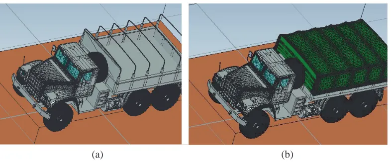
In this paper, as input data we consider the BSP obtained at wavelength 3 cm for horizontal polarization for two models of truck KRAZ. In order to show radar detectability reduction, we consider two KRAZ models with and without cloaking (Fig. 1). Both models were created with the help of 3D designer program.
For following estimation of the object detectability, it is necessary to calculate its backscattering pattern (BSP) when being placed on different types of background surface. In order to calculate the scattered field for the objects situated on different background surfaces, we use the technique proposed in [23]. In our considerations, the background surface is characterized by two parameters:
• Backscattering reflection which is conditioned by diffusive scattering at the surface irregularities. It creates “background” scattering signal, on which the object is to be detected. This parameter is not involved in calculation of the object’s BSP; it is taken into account below in statistical data processing.
• Specular reflection that influences the backscattering from the object due to rays that bounce between the object and the background surface.
Here we divide these two types of reflections and consider them as independent.
The former parameter is described with specific RCS of the surface backscattering σspec [28], and
(a) (b)
Figure 1. KRAZ models. (a) Model 1 — Source KRAZ model. (b) Model 2 — KRAZ model with cloaking.
Typically, calculation of the object BSP takes the most time (99% of the total detectability estimation time), at which for any required background surface type it requires separate long calculations. In order to optimize this process and to be able to analyze BSP for a wide range of possible background surfaces, the authors propose the calculation scheme based on decomposing the reflected field [29]. Thus, the scattered field can be divided into the following components:
1. The rays that are incident onto the object and reflected backwards;
2. The rays that are incident onto the object, then reflected towards the background surface and finally reflected towards the radar;
3. The rays that are incident onto the background surface, then reflected towards the object and finally reflected towards the radar;
4. The rays that are incident onto the background surface, then reflected towards the object, then reflected back to the background surface, and finally reflected towards the radar.
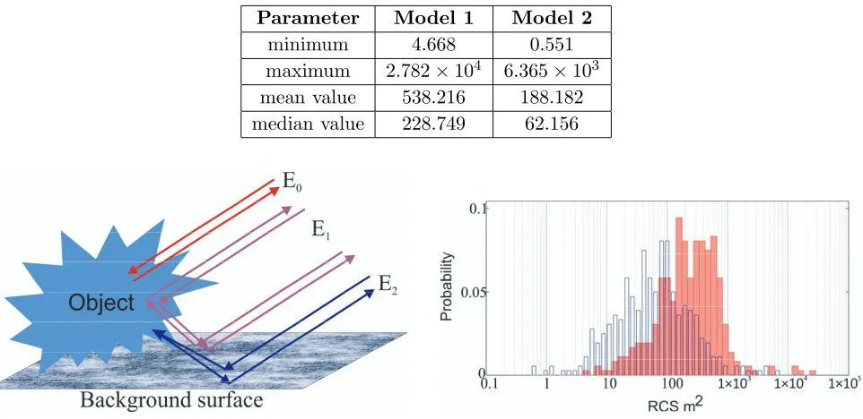
The reflected field E0 (see Fig. 3) created by the rays from case 1 does not interact with the background surface and thus, does not depend on the surface reflection coefficient (R). The reflected field E1 created by the rays from cases 2 and 3 interacts with the background surface only once, and hence it is proportional to R. Finally, the field component E2 is created by rays 4, and it interacts with the background surface twice, hence is proportional to the squared reflection coefficient R2. Fig. 3 schematically illustrates the above described interaction cases.
Thus, neglecting the further multiple reflections between the object and the ground, we can assume that the reflected field depends on the background surface reflectance R by the following law:
E(R) =E0+R·E1+R2·E2 (1)
Since the background surface is assumed to be infinite plane. The reflected field will be contributed only by the rays bouncing off the surface at the incidence angles that correspond to the radar elevation position. Hence in the case thatR is dependent on the incidence angle (e.g., by Fresnel formulae), the equation contains R for the given incidence angle θ.
Then we should perform simulation of the electromagnetic wave diffraction on radar target for the three cases:
1. The object is placed in a free space without any background surface, and the result is a complex value of the scattered fieldEAIR.
2. The object is over a perfectly electrically conducting (PEC) surface (the surface impedance is zero, and the reflectance isR=−1), and the result is a complex value of the scattered fieldEP EC.
[30]). It is pointed out that using inclined sidewalls of radar targets can reduce the component of the scattered field discussed above [3].
3. DETECTION PROBABILITY CALCULATION
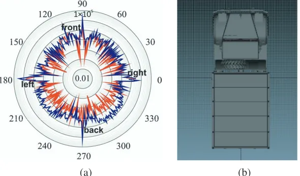
As a calculation result, we have RCS of the object on a specific background surface as a function of azimuth angle σi =σ(ϕi).
In Fig. 2, the dependencies for concrete background surface (lossless dielectric with permittivity ε= 5.5) are presented.
The radar can see object from different unpredictable directions. So, the RCS of the target is a random signal, and possibility to detect or not to detect the target can be considered from the statistical point of view. The content of this paragraph was briefly described in our conference paper [23], and now we present the extended version of this paper with some new results.
For our case, the obtained RCS angular dependencies have statistical parameters presented in Table 1.
It is important to mention that the mean and median values from Table 1 seem very large. That is why in our calculations we take into account the specular reflection from near-object part of the substrate. Another reason for the big values in Table 1 is the presence of some “corner reflectors” in the investigated model [3, 30].
For obtained data, we can draw histograms (see Fig. 4) where the solid bars designate data for model 1 and the empty bar for model 2. Here inx-axis, one can see the RCS values in logarithmic scale, iny-axis — the probability to obtain corresponding RCS value. Histograms in Fig. 4 are plotted with 50 pins.
(a) (b)
Table 1. RCS data in m2 from Fig. 2.
Parameter Model 1 Model 2
minimum 4.668 0.551
maximum 2.782×10⁴ 6.365×10³ mean value 538.216 188.182 median value 228.749 62.156
Figure 3. Object on background surface. Figure 4. Histograms for data in Fig. 2 (red filled columns — RCS of model 1, empty columns — RCS of model 2).
Of course, obtained RCS data can be approximated by some PDFs [24] for simplifying the following calculations. However, this can give significant errors in the case that BSP has many sharp highlights corresponding to specular reflections from different parts of the object. So, we can consider the obtained data without any approximations as a sum of delta functions which have peaks in the points corresponding to the calculated RCS valuesσi and have amplitudes 1/N (the probability to obtain RCS
valueσi) [23]:
Fobj(u) = N
i=1
δ(u−σi)/N (3)
In all discussions above we do not take into account the diffuse scattering from background surface. This is a rough surface, so its RCS can be considered as a random signal [31]. In our calculations, we suppose that this random signal satisfies Rayleigh PDF
Fbg(u, s) = (u/s2) exp(−u2/2s2) (4)
Here u is the random RCS value and sthe distribution parameter that corresponds to the median of the random value. In our calculations, we consider concrete as a rough surface. For the case under study (wavelength, incident angle), the specific RCS is equal toσsp=−46.7 dBm2 [20].
In the case that the radar lights the part of background surface with area SL, we obtain the distribution parameters in distribution of Eq. (4) for the given background surface as
s=σspSL. (5)
The illuminated part of background surface SL is determined by some parameters of radar station (distance to the station, beam width of radiation pattern).
given radar resolution (dr — the side of the square that is lighted by the radar beam on background surface). For this aim, we should define some threshold RCSσth. Usuallyσthis chosen from conditions
that false alarm probability is equal to value Pfa (often and in this work below Pfa = 10−4). False
alarm probabilityPfa is a probability that radar detects background. So, we have the following relation to obtain σth
Pfa =
∞
σth Fbg(u, s)du= 1− σth
0
Fbg(u, s)du (7)
Equation (7) leads toσth = (−ln(Pfa)2s2)1/2.
Now we can calculate the detection probability for the given radar resolution
Pdet=
∞
σthFobj+bg(u, s)du= 1− N
i=1
σth
0
Fbg(u−σi, s)du/N (8)
For the case that the background surface PDF has the form in Eq. (4), and the integrals in Eq. (8) can also be calculated in closed form and expressed in form
Pdet= 1−
N
i=1
1−exp
−(σth−σi)2
2s2
N = 1 N N i=1 exp
−(σth−σi)2
2s2
(9)
However, formula (9) needs some corrections. For calculations ofσth, we need the area of the illuminated
part of the background surface (see formula (5)). However, the investigated object shades some part of this surface. We designate this shaded part of the surface for each direction (with RCS σi) as Sish.
So, inPdet calculations for each direction (with RCSσi), we should useSL−Sish instead ofSL. Using
formula (5), we obtain the following expression forPdetcalculation
Pdet= 1 N N i=1 exp
− (σth−σi)2
2σ2
spSL−Sish 2
(10)
(a) (b)
For a certain direction, the visible area of the object can be larger than the illuminated part of the background surface Sish > SL — for this direction, the radar sees only the object. In this case, if the
RCS for lighted object part for this direction σi is larger thanσth, we add to the detection probability
a value 1/N. Using these considerations, we can write the final formulae for detection probability calculation in the following form
Pdet= 1 N
N
i=1
⎧ ⎪ ⎨ ⎪ ⎩
exp
− (σth−σi)2
2σ2
sp
SL−Sish 2
, Sish < SL;
η(σi−σth), Sish > SL;
(11)
Here η(x) is Heaviside function (unit step function): η(x) = 1 forx >0 and η(x) = 0 forx <0.
As a result of calculation by formula (11), one obtains the detection probability for the object on the given background 0< Pdet<1.
The above mentioned shadowed areaSish is calculated in the assumption of parallelepiped shape of
the object. Under any angle of view, three walls of the parallelepiped are seen. Suppose that we know heighth, lengthland widthw of the parallelepiped. Then, if it is illuminated by a source from thei-th direction with angle coordinatesθi from zenith and azimuthϕi from the direction along the length, the
area of the shadow can be calculated with the following formula:
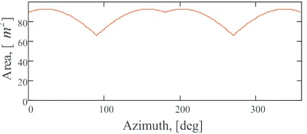
Sish(θi, ϕi) =h·tanθi·(l· |cosϕi|+w· |sinϕi|) +w·l (12) For example, Fig. 6 shows the dependence of the shadowed area on the azimuth angle for the object under consideration (model 1) at incidence angleθ= 40◦ from zenith. After cloaking (for model 2), the dimensions of the object are not changed significantly.
Figure 6. The shadowing area for the object under consideration (height h = 4.372 m, length l= 10.937 m and widthw= 4.559 m).
4. DETECTION PROBABILITY ANALYSIS
In fact, the detection probability for any specific object is a function of the lighted area of background surface SL and of the background specific RCS σsp. The lighted area of background surface SL is defined by the radar antenna pattern, and further we consider this area as square with sidedr (radar resolution), then SL=dr2.
The following dependence of detection probability on radar resolution (detection curves) for the background specific RCSσsp = 5.926 was obtained by technique described above.
Here one can see that for small radar resolutions, the detection probability is equal to Pdet= 1 — the object will be detected, and for big radar resolution the detection probability is equal to Pdet = 0 — the object is not visible on the background surface.
2 (hatch line).
(a) (b)
Figure 8. Dependence ofPdet on background specific RCS and on radar resolution for the (a) model 1 and (b) model 2. White color — Pdet= 1, black — Pdet= 0.
In order to understand how the detection probability Pdet behaves when varying both radar resolution and background level let’s plot two parametric dependences. In Fig. 8, the plot of such dependence is given in the form of level lines. From the plot one can see that when the radar resolution is below the object size (i.e., when the low part of formula (11) works), the detection probability does not depend on the resolution and remains constant. In the case of large resolution when background specific RCS is decreased by xdB and the radar resolution increased by xdB, then the detection probability remains the same.
So, the 0.5 level lines in the figure can be characterized by two numbers: “background specific RCS” that under small radar resolution provides 0.5 detection probability, and “effective object size”, at which the transition from the constant regime to the linear dependence regime occurs. The former parameter can be called “object specific RCS” (in Fig. 8. σ1 = 48.85 [dB] andσ2= 43.77 [dB]), and the latter — “object visible area” (in Fig. 8. L1 =L2= 33.74 [dBm]).
These parameters can be defined when we consider formula (11) as a function of two variables: object specific RCS σsp and radar resolutiondr(SL=dr2) —Pdet=Pdet(σsp, dr). The object specific RCS can be defined as the maximumσsp which the equation Pdet(σsp,0) = 1 satisfies for.
For example, for the considered objects in this paper, we have specific RCS σ1 = 48.85 [dB] for model 1 andσ2= 43.77 [dB] for model 2.
5. CONCLUSIONS
In this paper, we propose a methodology for calculating object detectability. For this purpose, we should estimate specific RCS of the object with the help of obtained formulae. This concept allows us to abstract from providing any specific background signal level and radar station parameters. From obtained values, we can calculate the object detection probability in the case of arbitrary background level and arbitrary radar resolution.
It should be noticed that the object specific RCS can be directly compared to the background specific RCS in order to make an immediate conclusion regarding detectability of the object on such a background when a sufficiently good radar is used (that have resolution smaller than the object size).
REFERENCES
1. Taravati, S. and A. Abdolali, “A new three-dimensional conical ground-plane cloak with homogeneous materials,” Progress In Electromagnetics Research M, Vol. 19, 91–104, 2011.
2. Wu, T. K., “From cloaking of conducting cylinder to RCS reduction/enhancement,”Radio Science
Meeting (Joint with AP-S Symposium), USNC-URSI, 133, IEEE, 2013.
3. Maslovskiy, A. and M. Legenkiy, “Geometrical techniques for reducing radar targets detectability,”
Proceedings of Conference on Radiophysics, Electronics and Biophysics YSC, Kharkiv, 2014. 4. Bouzidi, A. and T. Aguili, “RCS prediction from planar near-field measurements,” Progress In
Electromagnetics Research M, Vol. 22, 41–55, 2012.
5. Baussard, A., M. Rochdi, and A. Khenchaf, “PO/mec-based scattering model for complex objects on a sea surface,” Progress In Electromagnetics Research, Vol. 111, 229–251, 2011.
6. Borzov, A., A. Sokolov, and V. Suchkov, “Digital simulation of input signals of systems of a near radar-location from complex radar-tracking scenes,”Radio Electronics Magazine, 2004 (in Russian). 7. Youssef, N., “Radar cross section of complex targets,” Proceedings of the IEEE, Vol. 77, 722–734,
May 1989.
8. Sukharevsky, O. I., Electromagnetic Wave Scattering by Aerial and Ground Radar Objects, 288, Taylor & Francis Group, CRC Press, 2015.
9. De Adana, F. S., I. Gonzalez, O. Gutierrez, and M. F. Catedra, “Asymptotic method for analysis of RCS of arbitrary targets composed by dielectric and/or magnetic materials,” IEEE Proceedings — Radar, Sonar and Navigation, Vol. 150, No. 5, 375–378, 2003.
10. Ling, H., R.-C. Chou, and S.-W. Lee, “Shooting and bouncing rays: Calculating the RCS of an arbitrarily shaped cavity,” IEEE Trans. Antennas Propagat., Vol. 37, No. 2, 194–205, 1989. 11. Boag, E. M., “A fast physical optics (FPO) algorithm for double-bounce scattering,” IEEE Trans.
Antennas Propagat., Vol. 52, 205–212, 2004.
12. Boag, A., “A fast physical optics (FPO) algorithm for high frequency scattering,” IEEE Trans. Antennas Propagat., Vol. 52, 197–204, 2004.
13. Bhalla, R., H. Ling, J. Moore, D. J. Andersh, S. W. Lee, and J. Hughes, “3D scattering center representation of complex targets using the shooting and bouncing ray technique: A review,”IEEE Antennas Propagat. Mag., Vol. 40, 30–39, 1998.
14. Tao, Y. B., H. Lin, and H. J. Bao, “Kd-tree based fast ray tracing for RCS prediction,” Progress In Electromagnetics Research, Vol. 81, 329–341, 2008.
15. Gao, P. C., Y. B. Tao, Z. H. Bai, and H. Lin, “Mapping the sbr and tw-ildcs to heterogeneous cpu-gpu architecture for fast computation of electromagnetic scattering,” Progress In Electromagnetics Research, Vol. 122, 137–154, 2012.
16. Rius, M., M. Ferrando, and L. Jofre, “GRECO: Graphical electromagnetic computing for RCS prediction in real time,”IEEE Antennas Propagat. Mag., Vol. 35, 7–17, 1993.
algorithms polarization selection stationary ground objects,” Radio Electronics Magazine Vol. 4, 2013 (in Russian).
23. Legenkiy, M., A. Butrym, and M. Antyufeyeva, “Evaluation of on-ground object radar detectability reduction,”Proceedings of the Conference Mathematical Methods in Electromagnetic Theory, 254– 257, Dnipropetrovsk, Aug. 26–28, 2014.
24. Swerling, P., “Probability of detection for fluctuating targets,” IRE Transactions on Information Theory, Vol. 6, No. 2, 269–308, 1960.
25. Bergamaschi, L., G. D’Agostino, L. Giordani, G. Mana, M. Oddone, “The detection of signals buried in noise,” Data Analysis, Statistics and Probability, 1–12, 2013.
26. Shi, W., X.-W. Shi, and L. Xu, “RCS characterization of stealth target using χ2 distribution and lognormal distribution,”Progress In Electromagnetics Research M, Vol. 27, 1–10, 2012.
27. Zhuang, Y.-Q., C.-X Zhang, and X.-K. Zhang, “Accurate statistical modeling method for dynamic RCs,”PIERS Proceedings, 1135–1139, Guangzhou, Aug. 25–28, 2014.
28. Corbel, C., C. Bourlier, N. Pinel, and J. Chauveau, “Rough surface RCS measurements and simulations using the physical optics approximation,” IEEE Trans. Antennas Propagat., Vol. 61, No. 10, 5155–5165, Oct. 2013.
29. Maslovskiy, A. A. and M. N. Legenkiy, “Analysis of geometrical techniques for reducing radar detectability of on-ground targets,” Proceedings of the International Young Scientist Forum on Applied Physics, (YSF’2015), 1–4, Dnipropetrovsk, Sep. 29–Oct. 1, 2015.
30. Kobak, V., “Radar reflectors,” Soviet radio, 248, Moscow, 1975 (in Russian).