DIGITAL ARRAY MIMO RADAR AND ITS PERFORMANCE ANALYSIS
N. B. Sinha
Faculty of Electronics and Communication Engineering and Electronics and Instrumentation Engineering
College of Engineering & Management Kolaghat Purba-Medinipur, West Bengal 721171, India
R. Bera
Faculty of Electronics and Telecommunication Engineering Sikkim Manipal Institute of Technology
Sikkim Manipal University Majitar, Sikkim 737132, India
M. Mitra
Faculty of Electronics and Telecommunication Engineering Bengal Engineering and Science University
Shibpur, Howrah-11103, India
1. INTRODUCTION
It has been recently shown that multiple-input multiple-output (MIMO) [1, 2] antenna systems have the potential to dramatically improve the performance of communication systems over single antenna systems. Unlike beam forming, which presumes a high correlation between signals either transmitted or received by an array, the MIMO concept exploits the independence between signals at the array elements. In conventional radar, target scintillations are regarded as a nuisance parameter that degrades radar performance. The novelty of MIMO radar is that it takes the opposite view, namely, it capitalizes on target scintillations to improve the radar’s performance. The MIMO radar system under consideration consists of a transmit array with widely-spaced elements such that each views a different aspect of the target. It can overcome target RCS scintillations by transmitting different signals from several decor related transmitters. The received signal is a superposition of independently faded signals, and the average SNR of the received signal is more or less constant. This is in marked contrast to conventional radar, which under classical Swelling models suffers from large variations in the received power. Therefore the objectives of MIMO radar are the target resolution should have the higher as compared to conventional radar. Interference and clutter rejection should be the highest, RCS measurement accuracy should be the highest and multi-path and other environmental effects should be the minimum. But unfortunately MIMO technology alone cannot tackle all the problems solution.
Some notational conventions are:
* Lower case letters denote scalars, upper case letters denote matrices and boldface denote vectors.
* Subscript (c/)H denotes Hermitian transpose. * The operatorE(c/) denotes expectation. * The operatork(c/) denotes matrix norm.
* The operatorlmax(c/;c/) denotes the largest generalized eigenvalue of a pair of matrices.
* Let w be a beam forming weight vector. Then wli denotes the beam forming weight vector of theith user in thelth iteration. * The operator P(c/) returns the principal eigenvector of a matrix,
that is the eigenvector corresponding to its maximal eigenvalue.
2. MIMO CHANNEL DESCRIPTION
In quasi-static, independent and identically distributed (i.i.d.) frequency flat Rayleigh fading channels, MIMO target detection probability and receiver SNR increases as the number of antennas increases. This has been discussed in detail in later half as space diversity. In general, the sub channels of MIMO radar system are usually space selective because of the angle spread at the transmitter and/or receiver. Consider the multistatic nature of the radar where orthogonality is maintained in space domain using the condition
(Dt∗Dr)/R > λ/M (1) whereDtandDrare the transmit and receive antenna spacing,Ris the range between transmitter and receiver, λis the wavelength, M is the number of transmit antennas (assume thatM is large). In practice, for larger values of antenna spacing (1) the transmit antennas can fall into the grating lobes of the receive array, in this case, orthogonality is not realized. In a pure LOS situation, orthogonality can only be achieved for very small values of range R. This makes the DOD (Direction of departure) at the transmitter and DOA (Direction of arrival) at the receiver end uncorrelated. This makes the receiver robust against clutters and multipath effects. In other words, this is known as space diversity.The time-selective nature is caused by the Doppler spread and the frequency selective nature is caused by delay spread. The elementhp,qof the channel matrix provides the complex valued channel gain from transmitter antennap to receiver antenna q. Lethr(t) and
of unity. Let Ht(t, f) be the time-variant frequency responses for the channel before hitting the target and Hr(t, f) be the time-variant frequency responses for the channel before hitting the receiver. Using the distances and the coordinates of the target in spherical coordinates can be written as
Ht(t, f) = [(1/|r1|)]∗
ej(ωt−kr)
andHr(t, f) = [(σ/|r2|)]∗
ej(ωt−kr)
,
where ω = 2πf is the angular frequency of the transmitted signal and t is the time taken for the signal to reach the target from the transmitter,k= 2π(sinθ(cosφ)i+(sinθ∗sinϕ)j+cosϕ) is the freespace wavenumber of the signal and whereσ is the target reflectivity (which depends upon the receive look angles, θ the elevation and Φ, the azimuth). For simplicity one-dimensional ULAs of antennas with antenna spacing dtand dr. The channel matrix can be described the array steering and response vectors given by
aT(θT) = 1
√ P
1, e−j2ΠθT, . . . e−j2Π(P−1)θT
T
aR(θT) = 1
√ Q
1, e−j2ΠθR, . . . e−j2Π(Q−1)θR
T
Let gm,n(t, τ) be the time-varying impulse response of the (m, n)th sub-channel connecting the mth transmit antenna and the
nth receive antenna. Hence, gm,n(t, τ) = [σ/mod(r1)∗mod(r2)]∗ [ej(w−τ)−k(r1+r2)]∗a
T(θT)∗aR(θR). The complete channel matrix just before reaching the receiver is given Hm,n(t, τ) = gm,n(t, τ)∗hr(τ)∗
ht(τ).
The above relation is based on Kronecker product. Let sn(k) is a sequence of complex symbols of OSTBC transmitted by the nth transmit antenna with symbol period ofym(t) is the received signal at themth receive antenna, andym(k) is the sampled version ofym(t)with sampling period ofTs=T sym/γ, andγ is an integer number. Ifγ =t, then the sampling rate at the receiver is the same as the symbol rate at the transmitter. Using the time-frequency duality and convolution operation, the received signal can be finally represented as
ym(t) = N
n=1
∞
k=−∞
sn(k)hm,n(t, t−kTsym)+zm(t), where, m= 1,2,3
and the additive noise given by
andvm(t) is the zero-mean complex-valued white Gaussian noise with a two-sided power spectral density PR(t) =PT(t). The sampled version of the received signal at theqth receive antenna is given
ym(kTs) = N
n=1
∞
t=−∞
sn(l)hm,n(KTs, KTs−lγTs) +zm(KTs),
where m= 1,2, . . . M (3)
If we over sample the transmitted sequence sn{k} by inserting zeros between each {γ −1} symbolsn{k}, then the over sampled sequence
xn(K) can be defined as
xn(K) =
sn
k γ
, if
k γ
is integer
0 otherwise.
(4)
The signal vector received by the MIMO radar (after demodula-tion and matched filtering) is given by
ym(k) = N
n=1
∞
k=−∞
xn(k−1)hm,n(k, l) +zm(k),
where m= 1,2,3, . . . M (5)
where hm,n(k, l) = hm,n(kT s, lT s) and T s is the sampled version of
hm,n(t, τ) and zm(k) = zm(kT s) where T s is the sampled version of z(t). With the statistical properties of the discrete-time channel coefficientshm,n(k, l) and the additive noiseszm(k), the MIMO channel input-output can be fully characterized in the discrete time domain with high computational efficiency and no loss of information.
3. MIMO CHANNEL ASSUMPTIONS
Assumptions for the continuous-time physical channel of wideband MIMO wireless systems are as follows:
Assumption 1: The (p, q)th sub channel of gm,n(t, τ) a MIMO system is a wide-sense stationary uncorrelated scattering (WSSUS) [15, 16] rayleigh fading channel with a zero mean and autocorrelation given by
E
gm,n(t, τ)∗gm,n∗
t−ξ, T/ =J0(2Πfdξ)∗G(τ)∗δ
where (.)* is the conjugate operator d is the maximum Doppler
frequency, and G(Γ) is the power delay profile with ∞
−∞G(τ)dτ = 1,
where
G(τ) = K
i=1
σ2iδ(τ−τi) (7)
wherek is the number of total resolvable paths andσ is the power of the ith path with delay Γ. For example in wireless communication, the typical urban (TU), hilly terrain (HT), and equalization test (EQ) pro-files for GSM and EDGE systems [7] as well as the pedestrian and vehicular profiles for channel A and channel Bof cdma2000 and UMTS systems [8] have all been defined as discrete delayed Rayleigh fading paths, and almost all the path delays are not an integer multiple of their system’s symbol period domain. These statistics are further used to build a computationally efficient discrete-time MIMO channel simulator which is equivalent to its counterpart in the continuous-time domain in terms of various statistic measures.
Assumption 2: The space selectivity or (spatial correlation) between the (m, n)th subchannel Hm,n(t, T) and the (p, q)th subchannel Hp,q(t, T) is given by
E
Hm,n(t, τ)∗Hp,q∗
t−ξ, T/
=ρ(RXm,p)∗ρ(T Xn,q)∗J0(2Πfdξ)∗G(τ)8δ
T −T/ , (8) where ρ(RXm,p) is the receiver correlation Coefficient between receive antennas m and p with 0 =<abs(ρ(RXm,p)) =< ρ(RXm,p) = 1, and ρ(T Xn,q) is the transmitter correlation Coefficient between receive antennasnand
fading channels [6, 10]. However, it should be pointed out that the third sub assumption may not be extended to Rayleigh fading MIMO channels [11]. Spatial correlation coefficients are determined by the spatial arrangements of the transmit and receive antennas, the angle of arrival, the angular spread, etc. This can be calculated by mathematical formulas (6), (10) or obtained from experimental data.
4. DISCRETE-TIME MIMO CHANNEL MODEL FOR MIMO RADAR
4.1. Discrete Time Channel Model
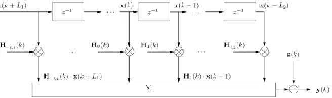
This discrete-time model based on MIMO Rayleigh fading channels and investigate the statistical properties of this MIMO channel in the discrete-time domain. These statistics are further used to build a computationally efficient discrete-time MIMO channel simulator, which is equivalent to its counterpart in the continuous-time domain in terms of various statistic measures depicted in Fig. 1.
response (FIR) channel. Without loss of generality, we assume that the coefficient index l is in the range of [−L1, L2], where L1 and L2
are nonnegative integers, and the total number of coefficients for the truncated FIR channel hm,n(k, L) is L with L <= L1 +L2, where
the equality is held if there are no discarded coefficients within the coefficient index range of (−L1,L2). Based on the above discussion
and (6) the input-output relationship of the MIMO channel in the discrete- time domain as follows:
y(K) = L2
l=−L1
Hl(K)·X(K−l) +Z(K) (9)
where
X(K) = [x1(k), x2(k), . . . , xn(k)]t
Z(k) = [z1(k), z2(k), . . . , zn(k)]t
Y(k) = [y1(k), y2(k), . . . , yn(k)]t
are the input vectors, noise vectors, and output vectors at the time instantk, respectively with (.)t represents transpose operator; Hl(K) is the LTs delayed channel matrix at time instant k and defined by
Hl(K) =
h1,1(K, l) · · · h1,N(K,l)
..
. . .. ...
hM,1(k, l) · · · hM,N(K, I)
It is noted that there are (MNL) stochastic channel coefficients, and an-element random noise vector in this MIMO Rayleigh fading model (10). Since all of them are complex valued Gaussian random variables, the first-order and second order statistics of the channel coefficients and the noise vector will be sufficient to fully characterize the MIMO channel. For the convenience of discussion, we define the MIMO channel coefficient vector
hvcc(k)={[h1,1(k), h1,2(k),. . .h1,N(k)]. . .[hM,1(k), hM,2(k),. . .hM,N(k)]}t wherehM,N(k) is the (m, n)th sub channel’s FIR coefficients at timek given by
hM,N(k) = [hM,N(k, L1). . . h1M,N(k, L2)] (10)
With the statistical properties of the discrete-time channel coefficients and the additive noises (including clutter, multipath effect and uncorrelated fading), the MIMO channel input-output can be fully characterized in the discrete time domain with high computational efficiency and no loss of information. It gives a deep insight into channel distortions caused by scattering components with different propagation delays k/ and discrete frequencies fn·fn/ =fn when considering two dimensional discrete time Fourier transform ofs(k/, fn).
In this case the four correlation functions h(k/, k), H(k/, k),
s(k/, fn), T(fn/, fn) are stochastic system functions representing discrete time impulse response, discrete time Transfer function, discrete time Doppler variant impulse response, discrete time Doppler variant transfer function. Generally, these stochastic system functions are described by the following autocorrelation functions:
rhh
k1/, k/2;k1, k2 := E
h∗
k/1, k1 h
k2/, k2 ,
rHH
fn/1, f2/n;k1, k2 := E
H∗
fn/1, k1 H
f2/n, k2 ,
rss
k1/, k2/;fn1, fn2 := E
s∗
k/1, fn1 s
k/2, fn2 ,
rT T
fn/1, fn/2;fn1, fn2 := E
T ∗
fn/1, fn1 T
fn/2, fn2 ,
In case of WSSUS (wide sense stationary uncorrelated scattering), the time difference (t2 −t1) in discrete domain is (K2 −K1) := K as
suchrhh(k/1, k
/
2;k1, k1+k) =δ(k2−k1)Shh(k1/, k), whereShh(k1/, k) is
called delayed cross-power spectral density. With this representation it becomes obvious that discrete time-variant impulse response h(k/, k) of WSSUS models has the characteristic properties of non-stationary white noise,clutter, multipath with respect to propagation delay K/, on the one hand, it is also stationary with respect to the time k, on the other hand. By analogy directly obtain autocorrelation function of T(fn/, fn). rT T(f/, f/ +v/;f1, f2) = δ(f2−f1)ST T(v/, f1), where
V1 =fn2−fn1 andST T(fn/1, v1) is called Doppler cross power spectral
density.
5. MODEL ERROR
Figure 2. Represents the quantized frequencies, time and phase approaches continuous model.
6. MODEL COMPLEXITY
This section illustrate the measurement of the computational complexity and the complexity of our proposed discrete-time MIMO channel simulation model is much lower than that of the conventional continuous-time simulation model based on the following aspects. i) The sampling rate of the discrete-time model is equal to the small positive integer. However, for the conventional continuous-time model, when the differential delay of multiple fading paths is very small compared to the symbol period, the sampling rate for simulation needs to be very high to implement the multiple fading paths. Sampling rate for the continuous-time model is the sampling computational complexity ratio of the discrete-time model to the continuous-time models is given by
ξn=
η ηc ×
100%
pass the input signals through the transmit and receive filters with extra computations. Moreover, to represent the small differential delay of multiple fading paths, the continuous-time model has to use a high sampling rate which makes the transmit and receive filters have large number of taps. This makes the computational complexity of the continuous-time model even higher than that of the discrete-time model. Unfortunately, an explicit ratio between these two models is unlikely to be obtained.
7. RESULTS AND SIMULATIONS 7.1. Detection Performance
A useful measure of radar fidelity is probability of detection (PD). Analytical forms of PD are obtained using radar detection theory originally described by Woodward [12]. It is not always feasible, or even possible, to find closed forms expressions forPD for every kind of radar. The detection performance comparison of radars thus becomes intractable in some cases. However, in this paper, we have used an alternative way to gauge the fidelity of radars by postulating an analogous communication system for radars (ACSR). Effective SER for this system have been calculated. Simple radar topologies have been used in this paper (as described above) to find closed form expressions for both techniques and to compare their simulation results. This has helped to obtain the parallel between probability of miss-detection (P M D = 1 −P D) of a radar and SER of the ACSR, by plotting graphs of each of these quantities against the received signal-to-noise ratio (SNR) for every kind of radar under test.
7.1.1. Symbol Error Rate
Using this model, the 1×1 SISO radar has only one channel in the ACSR. The 2×1 MISO and the 1×2 SIMO radars have two channels each and the 2×2 MIMO radar has four channels. This leads to the expressions for the received signal-to-noise ratios (SNRs) of each of these radars in terms of the respective channels:
SN RSISO = (|h1|)2
Em
δ2
n
SN RM ISO = 1
2(|h1|+|h2|)
2Em
δ2
n
SN RSIM O = (|h1|+|h2|)2
Em
δ2
SN RM IM O = 0.5(|h1|+|h2|+|h3|+|h4|)2
Em
δ2
n
where h1, h2, h3, h4 are the channels that are set-up in the respective
ACSRs andEm is the signal power while 2nis the noise power spectral density. Now the radars have been converted into communication systems. The SER of each of these systems is found using BPSK and QPSK modulation schemes. In BPSK with an additive white Gaussian noise (AWGN), the SER is given by Pb =Q(
2Em
δ2
n ), where Q(x) = 1/2erf c(x/1.414). The target can occupy any position in space defined by azimuth-elevation space θ= [0, pi] and Φ defined by = [0,2pi). Letp(θ, Φ) be the probability density function of the target positions. Then the SERs of each of the four radar systems are given, using BPSK, by:
PSISO= 2Π
0
Π
0
Q2(|h1|)2
Eb
Nq
p(θ, ϕ) sinθdθdϕ
PM ISO= 2Π
0
Π
0
Q(|h1|+|h2|)2
Eb
Nq
p(θ, ϕ) sinθdθdϕ
PSIM O= 2Π
0
Π
0
Q2(|h1|+|h2|)2
Eb
Nq
p(θ, ϕ) sinθdθdϕ
PM IM O= 2Π
0
Π
0
Q(|h1|+|h2|+|h3|+|h4|)2
Eb
Nq
p(θ, ϕ) sinθdθdϕ
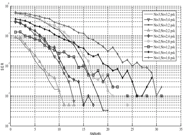
By assuming uniform probability distribution for the target and an arbitrary fading probability distribution for the radar target reflectivity over all the azimuth-elevation space, the integrals in the above equations are evaluated numerically. Fig. 4 shows the results of SER performances. For all SNR levels, MIMO system has the least SER, and hence the highest probability of detection because the lower the error in the received signals, the higher is the detection.
0 5 10 15 20 25 30 35 10-4
10-3 10-2 10-1 100
SNR(dB)
SE
R
Nt=3;Nr=3;2 psk Nt=3;Nr=3;4 psk Nt=3;Nr=3;2 psk Nt=2;Nr=2;2 psk Nt=2;Nr=2;4 psk Nt=2;Nr=2;8 psk Nt=1;Nr=1;2 psk Nt=1;Nr=1;4 psk Nt=1;Nr=1;8 psk
Figure 3. In discrete time model the symbol error rate is being calculated with respect to SNR value.
Figure 4. Channel coefficients for digital array 3 by 3 MIMO radar with respect to contour profile.
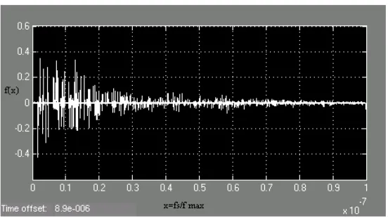
Figure 5. The power spectral density of the Discrete time digital array MIMO radar.
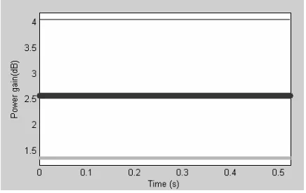
Figure 6. Dynamic variation in absolute power gain of the three parallel SISO channels.
channel coefficients of the discrete time MIMO channel.
The contour plot determines the dependencies with respect to the time between the channel coefficients of the discrete time MIMO channel.
7.1.2. PSD at the Receiver
is used for MIMO radar test. Also the target is assumed to be modulating passive object. Thus, the space diversity is being taken into action to have better outlook with respect to multistatic radar.
7.1.3. Time Response ofthe Channel Coefficient of3∗3 MIMO The power level at the transmitter considering the multistatic nature of radar depending upon the position of the target based on SNR value at the receiver. The three parallel channels are notified which indicate that diversity in power is uniform with respect to gain level. Thus, individual antennas will behave in uncorrelated manner with respect to the orthogonality due to OSTBC and antenna spacing.
8. CONCLUSION
linearly. However, the scaling rates for all the three cases are dependent on the spatial correlation coefficients (the less correlation, the larger the scaling rate). This observations are therefore valuable extensions to the Shannon channel capacity results of triply selective MIMO Rayleigh fading channels from the special case of quasistatic i.i.d. flat Rayleigh fading MIMO channels in multistatic radar systems.
REFERENCES
1. Foschini, G. J., “Layered space-time architecture for wireless communication in a fading environment when using multiple antennas,”Bell Labs Technical Journal, Vol. 1, 41–59, 1996. 2. Foschini, G. J. and M. J. Gans, “On the limits of wireless
communications in a fading environment when using multiple antennas,”Wireless Pers. Commun., Vol. 6, 311–335, 1998. 3. Fishler, E., A. Haimovich, R. Blum, L. Cimini, D. Chizhik, and
R. Valenzuela, “MIMO radar: An idea whose time has come,” Proc. ofthe IEEE Int. Conf. on Radar, Philadelphia, PA, April 2004.
4. Fishler, E., A. Haimowich, R. Blum, L. Cimini, D. Chizhik, and R. Valenzuela, “Statistical MIMO radar,”12th Conf. in Adaptive Sensor Array Processing, 2004.
5. Khan, H. A., D. J. Edwards, W. Q. Malik, and C. J. Stevens, “Ultra wideband multiple-input multiple-output radars,” IEEE International Radar Conference, Arlington, Virginia, USA, 2005. 6. Johnson, D. and D. Dudgeon, Array Signal Processing,
Prentice-Hall, Englewood Cliffs, NJ, 1993.
7. “Radio transmission and reception,” ETSI. GSM 05.05, ETSI EN 300 910 V8.5.1, 2000.
8. “Selection procedure for the choice of radio transmission technologies of UMTS,” UMTS, UMTS 30.03 version 3.2.0 ETSI, 1998.
9. Chuah, C. N., D. N. C. Tse, J. M. Kahn, and R. A. Valenzuela, “Capacity scaling in MIMOwireless systems under correlated fading,” IEEE Trans. Inform. Theory, Vol. 48, 637–650, Mar. 2002.
12. Jeruchim, M. C., P. Balaban, and K. S. Shanmugan, Simulation ofCommunication Systems: Modeling, Methodology, and Techniques, 2nd edition, Kluwer, Berlin, Germany, 2000.
13. Woodward, P. M., Probability and Information Theory with Application to Radar, Artech House, MA, 1953.
14. Xiao, C., et al., “A discrete-time model for triply selective MIMO rayleigh fading channels,”IEEE Transactions on Wireless Communications, Vol. 3, No. 5, September 2004.
15. Bello, P. A., “Characterization of randomly time-variant linear channels,” IEEE Trans. Commun. Syst., Vol. 11, 360–393, Dec. 1963.
16. Parsons, J. D., The Mobile Radio Propagation Channel, 2nd edition, Wiley, New York, 2000.
17. Reed, J. H., “Software radio — A modern approach to radio engineering,” Smart Antenna, Chapter 6, Pearson Education, 2006.
18. Sarkar, T. K., M. C. Wicks, M. Salazar-Palma, and R. J. Bonneau, Smart Antennas, Wiley Series in Microwave and Optical Engineering, 2003.