Testing Genetic Pleiotropy with GWAS Summary Statistics for Marginal and Conditional Analyses

(1)

HIGHLIGHTED ARTICLE

| INVESTIGATION

Testing Genetic Pleiotropy with GWAS Summary

Statistics for Marginal and Conditional Analyses

Yangqing Deng and Wei Pan1

Division of Biostatistics, University of Minnesota, Minneapolis, Minnesota 55455

ABSTRACTThere is growing interest in testing genetic pleiotropy, which is when a single genetic variant inﬂuences multiple traits.

Several methods have been proposed; however, these methods have some limitations. First, all the proposed methods are based on the use of individual-level genotype and phenotype data; in contrast, for logistical, and other, reasons, summary statistics of univariate SNP-trait associations are typically only available based on meta- or mega-analyzed large genome-wide association study (GWAS) data. Second, existing tests are based on marginal pleiotropy, which cannot distinguish between direct and indirect associations of a single genetic variant with multiple traits due to correlations among the traits. Hence, it is useful to consider conditional analysis, in which a subset of traits is adjusted for another subset of traits. For example, in spite of substantial lowering of low-density lipoprotein cholesterol (LDL) with statin therapy, some patients still maintain high residual cardiovascular risk, and, for these patients, it might be helpful to reduce their triglyceride (TG) level. For this purpose, in order to identify new therapeutic targets, it would be useful to identify genetic variants with pleiotropic effects on LDL and TG after adjusting the latter for LDL; otherwise, a pleiotropic effect of a genetic variant detected by a marginal model could simply be due to its association with LDL only, given the well-known correlation between the two types of lipids. Here, we develop a new pleiotropy testing procedure based only on GWAS summary statistics that can be applied for both marginal analysis and conditional analysis. Although the main technical development is based on published union-intersection testing methods, care is needed in specifying conditional models to avoid invalid statistical estimation and inference. In addition to the previously used likelihood ratio test, we also propose using generalized estimating equations under the working independence model for robust inference. We provide numerical examples based on both simulated and real data, including two large lipid GWAS summary association datasets based on 100,000 and189,000 samples, respectively, to demonstrate the difference between marginal and conditional analyses, as well as the effectiveness of our new approach.

KEYWORDSGEE; likelihood ratio test; multiple-trait association testing; structural equation models; union-intersection test; Wald test

T

HERE has been a growing interest in testing genetic pleiotropy, which is when a single genetic variant (or gene) inﬂuences multiple traits (Solovieff et al. 2013). As pointed out by Schaid et al. (2016), detecting pleiotropy may shed light on the underlying biological mechanism of a genetic association, with important implications for thera-peutic development, such as drug repurposing. Testing plei-otropy can be also useful in checking an assumption (i.e., no pleiotropic effects of a genetic instrument variable on both a risk factor/exposure and an outcome) imposed by Mendelian randomization for causal inference. There is accumulating empirical evidence to support pervasive pleiotropy for

com-plex diseases and traits (Cotsapaset al.2011; Q. Wanget al. 2015). Leveraging pleiotropy in GWAS with multiple traits may boost statistical power in detecting genetic associations (Chung et al.2014) as well as improving genetic risk pre-diction (Li et al.2014). Most existing methods for analysis of multiple traits test on a global null hypothesis that none of the traits is associated with a genetic variant, which, if re-jected, cannot tell whether the genetic variant is associated with only one or with two or more traits (e.g., Y. Wanget al. 2015; Kim et al.2016; Z. Wanget al.2016 and references therein). In pleiotropy testing, the target of interest is not the global null hypothesis, but rather that the genetic variant is associated with no more than one trait. A simple approach wouldﬁrst conduct a univariate association test on each trait separately, then check whether two or more P-values are signiﬁcant after a proper multiple testing adjustment. As shown in a later example, this naïve approach is often too

Manuscript received July 4, 2017; accepted for publication September 29, 2017; published Early Online October 2, 2017.

1_{Corresponding author: Division of Biostatistics, University of Minnesota,}

(2)

low powered due to the univariate nature of this test. Accord-ingly, some methods have been developed to test pleiotropy. Cotsapas et al. (2011) developed a cross-phenotype meta-analysis (CPMA) method to test pleiotropy using summary sta-tistics, which seems straightforward, but requires that we already know of the existence of one significant association, which may not be practical. In addition, it imposes a strong parametric as-sumption on the distribution of the marginal associationP-values under the alternative hypothesis, which may lead to loss of power when the assumption does not hold. Alternatively, other methods explore which of the multiple traits are associated (Stephens 2013; Majumdaret al.2016). Schaidet al.(2016) not only nicely surveyed existing methods, but also proposed a new and rigorous pleiotropy test based on the intersection-union testing approach (Berger 1997) with individual-level genotype and phenotype data. However, Schaidet al.(2016) focused mainly on the mar-ginal analysis of each trait (with possible covariates). Sometimes, a single-nucleotide polymorphism (SNP) might influence a trait through some intermediate traits, which means the effect on the trait is indirect. It is well-known that marginal analysis cannot distinguish direct and indirect effects. In contrast, conditional analysis can, and thus might be more useful. For example, al-though low-density lipoprotein (LDL) cholesterol remains the primary treatment target to reduce cardiovascular disease (CVD) risk, it has been shown that high triglyceride (TG) level is a possible independent risk factor for CVD, even in patients with treatment-controlled LDL levels (Boekholdt et al. 2012; Sampson et al. 2012; Doet al. 2013; Toth 2016). Hence, to identify new targets for new therapy to reduce levels of TG or other non-LDL lipids, it is more desirable to detect genetic vari-ants associated with TG and non-LDL lipids after adjusting for LDL; otherwise, due to the known correlations among various lipids, an identified association, say with TG, could simply be due to an indirect effect through LDL.

Importantly, since we most often have summary association statistics only from meta- or mega-analyzed large genome-wide association study (GWAS) data, rather than individual level data, it would be useful to have a pleiotropy test applicable to GWAS summary statistics. With these considerations, weﬁrst propose extending the likelihood-ratio test (LRT) of Schaidet al.(2016) with individual-level data to that with only summary statistics for marginal analysis with possible covariates (i.e., exogenous variables). Next, for either individual-level GWAS data or sum-mary statistics, we develop a new testing procedure for condi-tional analysis with some traits as both responses and predictors in multiple conditional regression equations; care has to be taken in this extension to avoid biased estimation and inference. To test a composite null hypothesis, we adopt the union-intersection testing strategy as used in Schaidet al.(2016). In particular, we consider conditional regression equations with some traits as both responses and predictors, for which, in addition to extend-ing the LRT of Schaidet al.(2016), for simplicity and robust-ness, we propose using the Wald test in generalized estimating equations (GEE) with the working independence model.

We will use simulations to show the feasibility of marginal or conditional analysis with summary statistics as well as the difference

between marginal and conditional analyses. We will also apply the methods to real data to further demonstrate these points.

Methods

Marginal analysis with individual level data

In this section, we give a brief review of the pleiotropy test of Schaidet al.(2016). Throughout this paper, a marginal anal-ysis is deﬁned as one in which no proper subset of traits is used as response in some regression models and as covariate in some other regression models. Hence, a marginal analysis allows the adjustment for nontrait covariates like multiple SNPs. Correspondingly, a conditional analysis is based on multiple regression models including some traits as both re-sponses and covariates.

Suppose that the individual level data containptraits andq SNPs (or other covariates) fornsubjects. As mentioned by Schaid et al.(2016), the covariates may be either trait-varying or not trait-varying. For simplicity, we just assume the same q SNPs across different traits. Let Yj¼ ðyj1;yj2; :::;yjnÞ9 denote the

measuredjth trait, andXk¼ ðxk1;xk2; :::;xknÞ9denote thekth

SNP for allnsubjects. Assume they are all centered at 0. The regression model can be expressed as

Y¼Xbþe，

where

Y¼Y19 . . . Yp9

9;

X¼X1* . . . Xq*

;

Xk*¼Ip5Xk;

b¼b19 . . . bq9

9;

bk¼bk1 . . . bkp

9;

e Nð0;VÞ;and

V¼S5In:

Inis an3nidentity matrix,5is the Kronecker product, and

the p3p matrix S is the covariance matrix for the errors within subjects. All theqSNPs are adjusted for in this model. Suppose the null hypothesis is H0: at most one of the

parameters b11; ..., b1p is nonzero. It is equivalent to test

whether one of the followingpþ1 tests holds:

Hj0:b1j6¼0; b1j1¼0ðj16¼jÞand

H00:b1j¼0ðj¼1;2; :::;pÞ

Let V0¼ ðIp 0Þ be a p3ðpqÞ matrix. Denote the matrix

(3)

equivalent to Vjb¼0:Schaidet al.(2016) proposed using

the test statistic

tj¼Y~9X~ðX~9X~Þ21Vj9½VjðX~9X~Þ21Vj921VjðX~9X~Þ21X~9Y;~

whereX~¼

V21=2_X

1* . . . V21=2Xq*

;Y~¼V21=2_Y;

and V¼S5In: Use ordinary least squares to estimate b; and

thenScan be estimated using the residuals. According to Schaidet al.(2016),T¼ min

j¼0;:::;ptjis the LRT

statistic forH0:

Since the null distribution ofTis complicated, they tested H0in two stages. Theﬁrst stage usest0;and the second stage

uses

T1¼ min

j¼1;:::;ptj:

t0asymptotically followsx2pwhenb1¼0:T1asymptotically

followsx2

p21when only one ofb11;...,b1pis nonzero. Reject

H0only ift0.x2pðaÞandT1.x2p21ðaÞ:

Marginal analysis with summary statistics

In this section, we describe a few steps to calculate the pre-vious test statistics based only on GWAS summary statistics.

1. If we have eachb^kj;the marginal effect ofXkonYj;and its

variance varcðb^kjÞ; as well as some reference panel and

summary statistics of null SNPs (i.e., not associated with any traits), we can estimateXk9Yj;Xk19Xk2andYj19Yj2:If we only have Z-statistics, we can regard them as ^bkj’s and

assumevarcðb^kjÞ ¼1:This approach turns out not to inﬂ

u-ence the result for marginal analysis, but may change the result for conditional analysis.

1a. Suppose we have individual level data Xref _¼

ðXref

1 ⋯ XrefqÞ centered at 0 from some

refer-ence panel for the SNPs of interest, where Xref

iis

the ith SNP for nref _{subjects. We can estimate}

ðXk19Xk2Þq3q=n by ðX

ref

k19X

ref

k2Þq3q=nref; and

ðXk19Xk2Þq3q by ðXrefk19X

ref

k2Þq3qn=nref: Note that

multiplying ðXk19Xk2Þq3q by a constant does not

affect the test results, so we do not really have to use the scalarn=nref_:_{For marginal analysis with}

only one SNP, we can simply assume X19X1 is 1.

1b. EstimateYj9Yj using

Yj9Yj2X19X1b^1j2¼ ðn21ÞX19X1varcð^b1jÞ;

where we plug in our estimate ofX19X1 asX19X1:

1c. Suppose we have Z-statisticsZjfor marginal analysis

offfiffiffiffiffiffiffiffiffiffiffiffiffiffiffiffiffiffiffiffiffiffiffiffiffiffiYjwith many null SNPs. We can estimateYj19Yj2as Yj19Yj1Yj29Yj2

p

corðZj1;Zj2Þ when j16¼j2; using the idea of Kimet al.(2015) and Kwak and Pan (2016, 2017) that

Yj19Yj2

ffiffiffiffiffiffiffiffiffiffiffiffiffiffiffiffiffiffiffiffiffiffiffiffiffiffi

Yj19Yj1Yj29Yj2

p corðYj1;Yj2Þ corðZj1;Zj2Þ:

1d. EstimateXk9Yjusing

Xk9Yj¼^bkjXk9Xk:

2. Estimate the ordinary least squares (OLS) estimate ^

B¼_b^₁ . . . ^bq

Note that the OLS estimate and the GLS estimate are the same when there is no trait-speciﬁc covariate, which is true in our current scenario. The for-mula is simply

vecð^BÞ ¼ ðX9XÞ21X9Y:

X9YandX9Xcan be obtained by

X9Y¼X19Y1. . .X19YpX29Y1. . .X29Yp. . .Xq9Y1. . .Xq9Yp

9;

X9X＝Xk19Xk2_q₃_q5Ip:

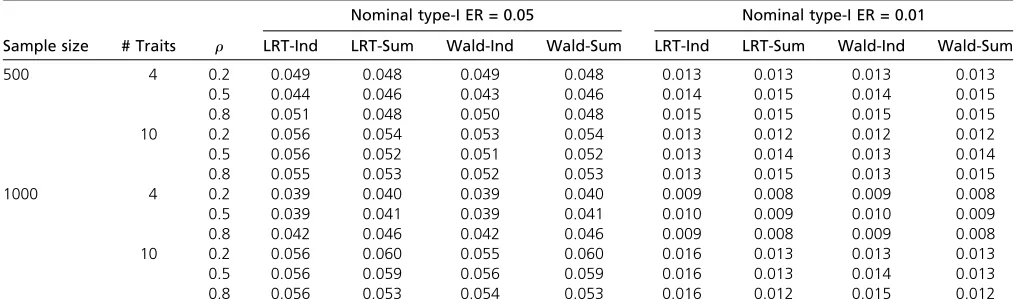
3. EstimateS^ from the residuals.S^ can be expressed as Table 1 Type I errors for set-up A withb11¼1;b1j¼0 ðj6¼1Þ

Sample size # Traits r

Nominal type-I ER = 0.05 Nominal type-I ER = 0.01

LRT-Ind LRT-Sum Wald-Ind Wald-Sum LRT-Ind LRT-Sum Wald-Ind Wald-Sum

500 4 0.2 0.049 0.048 0.049 0.048 0.013 0.013 0.013 0.013

0.5 0.044 0.046 0.043 0.046 0.014 0.015 0.014 0.015

0.8 0.051 0.048 0.050 0.048 0.015 0.015 0.015 0.015

10 0.2 0.056 0.054 0.053 0.054 0.013 0.012 0.012 0.012

0.5 0.056 0.052 0.051 0.052 0.013 0.014 0.013 0.014

0.8 0.055 0.053 0.052 0.053 0.013 0.015 0.013 0.015

1000 4 0.2 0.039 0.040 0.039 0.040 0.009 0.008 0.009 0.008

0.5 0.039 0.041 0.039 0.041 0.010 0.009 0.010 0.009

0.8 0.042 0.046 0.042 0.046 0.009 0.008 0.009 0.008

10 0.2 0.056 0.060 0.055 0.060 0.016 0.013 0.013 0.013

0.5 0.056 0.059 0.056 0.059 0.016 0.013 0.014 0.013

(4)

^ S¼ 1

n2pq

Xn

i¼1 _{_}

Yi2B^Xi_Yi_2B^Xi_9:

whereY_i¼ ðy1i;y2i; :::;ypiÞ9andX_i¼ ðx1i;x2i; :::;xqiÞ9:By

simple algebra, we have

ðn2pqÞS^ ¼X n

i¼1 _

YiYi_9þB^ X n

i¼1 _ XiXi_9

^ B9

2B^Xn i¼1 _ XiYi_9 2

^ BXn

i¼1 _ XiYi_9

₉

;

Xn

i¼1 _

YiYi_9¼ ðYj19Yj2Þp3p;

Xn

i¼1 _

XiXi_9¼Xk19Xk2_q₃_q; and

Xn

i¼1 _

XiYi_9¼ ðXk9YjÞq3p:

Thus, we can obtainS^ usingXk9Yj;Xk19Xk2;Yj19Yj2andB:^ ThenV^ is simplyS^5In:

4. Now we only need to knowX~9X~andX~9Y:~ By simple alge-bra, and replacingVwithV;^ we have

~

X9X~¼Xk19Xk2_q₃_q5S^21;

~

X9Y~¼_ð_X_1*₉_V^21_Y_Þ₉_⋯_ð_Xq_*₉_V^21_Y_Þ₉₉_;

ðXk*₉_V^21_Y_Þ₉_¼ P p

j¼1

a1jXk9Yj ⋯ P p

j¼1

apjXk9Yj;

where akjis theðk;jÞth entry ofV^ 21

¼S^215In:Finally,

we can calculate the statistics

tj¼Y~9X~ðX~9X~Þ21Vj9½VjðX~9X~Þ21Vj921VjðX~9X~Þ21X~9Y:~

The remaining testing procedure is the same as that in the previous section.

Conditional analysis with LRTs

For conditional analysis, we consider adjusting for a proper subset of the traits in the regression models for another (non-intersecting) subset of the traits as the responses. The derivation of the above LRT can still be carried out. If we have individual level data, the original method of Schaidet al.(2016) should allow incorporation of some traits as trait-speciﬁc covariates, though their R package “pleio” allows taking only one SNP without any other covariates. If we only have summary statis-tics, similar to what was done in Deng and Pan (2017), we can follow the previous idea to derive a similar procedure.

Now, the matrix notation we use is

Y¼XyG

b

a

þe;

e Nð0;VÞ;

V¼S5In:

Yis the same as before, while

Xy¼

X1* . . . Xq* Y1* . . . Yp*

;

Xk*¼Ip5Xk;

Yj*_¼_Ip₅_Yj:

Thus,Xy is aðnpÞ3ðpqþp2Þ design matrix combining the

information ofXandY:XyGis a reﬁned version ofXy with

ðpqþp2₂_p_Þ_columns.

Gis aðpqþp2_Þ₃_ð_pq_þ_p2₂_p_Þ_{matrix obtained by}

delet-ing theðpqþ1Þth,ðpqþpþ2Þth, ...,ðpqþp2_Þ_{th columns of}

an identity matrix of orderpqþp2_:_{The purpose of multiplying}

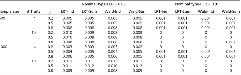
Table 2 Type I errors for set-up B withb11¼0;b1j¼0ðj6¼1Þ

Sample size # Traits r

500 4 0.2 0.005 0.005 0.005 0.005 0.001 0.001 0.001 0.001

0.5 0.005 0.005 0.005 0.005 0.001 0.001 0.001 0.001

0.8 0.008 0.008 0.008 0.008 0.001 0.001 0.001 0.001

10 0.2 0.010 0.009 0.008 0.009 0 0 0 0

0.5 0.010 0.008 0.008 0.008 0 0 0 0

0.8 0.008 0.008 0.008 0.008 0 0 0 0.001

1000 4 0.2 0.003 0.003 0.003 0.002 0 0 0 0

0.5 0.004 0.005 0.004 0.005 0.001 0.001 0.001 0.001

0.8 0.006 0.005 0.006 0.005 0.001 0.001 0.001 0.001

10 0.2 0.013 0.011 0.012 0.011 0 0 0 0

0.5 0.011 0.012 0.010 0.012 0 0 0 0

(5)

Xy byGis to delete the corresponding columns ofXy so that

the model will be YjX1þ:::þXqþY1þ:::þYj21þ

Yjþ1þ:::þYpinstead ofYjX1þ:::þXqþY1þ:::þYp:

Denote the effect of thekth SNP on thejth trait bybkjand

the lth trait on the jth trait by alj: b¼

b19 . . . bq9

9; bk¼

bk1 . . . bkp

9: Vector a is pðp21Þ dimen-sional. a¼ ða19 . . . ap9Þ9; al¼

al1 . . . al;l21

al;lþ1. . . alp

9:

The detailed testing procedure is described below. Now the test statistic is

tj¼Y~9X~ðX~9X~Þ21Vj9½VjðX~9X~Þ21Vj921VjðX~9X~Þ21X~9Y;~

whereX~¼V21=2XyG;~Y¼V21=2Y:Besides, in the new

sce-nario,Vjisðp21Þ3ðpqþp22pÞrather thanðp21Þ3ðpqÞ:

We only need to add zeros to the right of the previousVj:

Following the previous procedure, we can gettj’s using a

few steps:

1. EstimateXk9Yj;Xk19Xk2andYj19Yj2using the summary sta-tistics, reference panels, and null SNPs. The procedure is described in point (1) in the previous section.

2. Estimate the OLS estimateB^v by

^

Bv¼ ðG9Xy9XyGÞ21G9Xy9Y:

Denote

X1* . . . Xq*

by X* _and

Y1* . . . Yp*

by Y*:X_y9Y_andX_y9X_y_{can be obtained by}

Xy9Y¼

ðX*9YÞ9 ðY*9YÞ99;

Xy9Xy¼

X*9X* X*9Y* Y*9X* Y*9Y*

:

Following ideas similar to those presented above, we can easily get

X*₉_Y_¼_X

19Y1. . .X19YpX29Y1. . .X29Yp. . .Xq9Y1. . .Xq9Yp

9;

Y*9Y¼Y₁9Y₁. . .Y₁9YpY₂9Y₁. . .Y₂9Yp. . .Yp9Y₁. . .Yp9Yp9;

X*₉_X*_＝_Xk1₉_Xk2

q3q5Ip;

X*9Y*＝ðXk9YjÞ

q3p5Ip; and

Y*₉_Y*_＝_ð_Yj1₉_Yj2_Þ

p3p5Ip:

3. EstimateS^ from the residuals.S^ can be expressed as

^

S¼ 1

n2pðqþp21Þ

Xn

i¼1 _{_}

Yi2B^Xi_Yi_2B^Xi_9;

whereY_i¼ ðy1i;y2i; :::;ypiÞ9andX_i¼ ðx1i; :::;xqi;y1i; :::;

ypiÞ9: Here,X_i includes both SNPs and traits. Note

that B^¼ ðb^1. . . ^bqa^1*. . . ^ap*Þ; while B^v¼ ðb^19. . .

^

bq9a^19. . . ^ap9Þ: a^j*’s are p dimensional vectors

obtained by adding a 0 element between the ðj21Þth and jth elements of a^j’s. Hence, we can

get B^fromB^v:By simple algebra, we have

½n2pðqþp21ÞS^ ¼X n

i¼1 _

YiYi_9þB^ X n

i¼1 _ XiXi_9

^ B9

2B^Xn i¼1 _ XiYi_9 2

^ BXn

i¼1 _ XiYi_9

₉

;

Xn

i¼1 _

YiYi_9¼ ðYj19Yj2Þp3p;

Xn

i¼1 _ XiXi_9¼

Xk19Xk2_q₃_q ðXk9YjÞq3p ðYj9XkÞp3q ðYj19Yj2Þp3p

!

;and

Xn

i¼1 _

XiYi_9¼ Xk9Yj

q3p9

Yj19Yj2

p3p

₉

:

Thus we can obtain S^ usingXk9Yj; Xk19Xk2;Yj19Yj2 and B^v: Then,V^ is simplyS^5In:

4. Again, we only need to know ~X9X~ and X~9Y:~ By simple algebra, and replacingVwithV;^ we have

~ X9X~¼G9

! 5S^21

!

G;

Xk1*₉_V^21_Xk2*_¼ 0

@a11Xk19Xk2 _⋱ 0

0 appXk19Xk2

1 A_;

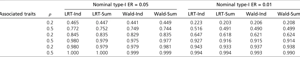
Table 3 Power

# Associated traits r

2 0.2 0.465 0.447 0.441 0.449 0.223 0.203 0.206 0.208

0.5 0.772 0.752 0.749 0.744 0.516 0.491 0.490 0.499

3 0.2 0.845 0.835 0.829 0.835 0.647 0.618 0.621 0.624

0.5 0.980 0.979 0.975 0.977 0.927 0.916 0.915 0.914

5 0.2 0.980 0.979 0.979 0.981 0.943 0.933 0.937 0.938

(6)

Yj1*₉_V^21_Yj2*_¼ 0

@a11Yj19Yj2 _⋱ 0

0 appYj19Yj2

1 A_; _and

Xk*₉_V^21_Yj*_¼ 0

@a11Xk9Yj _⋱ 0

0 appXk9Yj

1 A_;

where aljis theðl;jÞth entry ofV^ 21

¼S^215In:As forX~9Y;~

we can derive

~

X9Y~¼G9_ð_X_1*₉_V^21_Y_Þ₉

⋯ðXq*9V^21YÞ9ðY_1*9V^21YÞ9⋯

ðYp*₉_V^21_Y_Þ₉₉_;

ðXk*9V^21YÞ9¼ P p

j¼1

a1jXk9Yj ⋯ Pp j¼1

apjXk9Yj

;

ðYj1*9V^21YÞ9¼ P p

j2¼1

a1j2Yj19Yj2 ⋯ Pp

j2¼1

apj2Yj19Yj2

:

Hence, we can get everything we need as long as we can estimateXk9Yj;Xk19Xk2andYj19Yj2:These estimates are obtained in step (1).

We can modify the model with a different form of G: One model we are interested in is YiX1þ:::þXqþ

Y1þ:::þYi21: To ﬁt this model, we let G be a

ðpqþp2_Þ₃_ð_pq_þ_p_ð_p₂₁_Þ₌₂_Þ_{matrix. It is obtained by}

com-bining the ﬁrst pq columns of an identity matrix of order pqþp2 _{with columns} _pq_þ_ip_þ_j; _where _i_¼_{1; :::;} _p₂_1;

j¼1; :::; i: Following this notation, vector a becomes

a¼ ða29 . . . ap9Þ9; whereaj¼ ðaj1 . . . aj;j21Þ9:

Our speciﬁed model for conditional analysis is a so-called recursive system: (1) it contains a hierarchical model with some traits as predictors for other traits, but not otherwise, and (2) the error terms in the different regression equations are independent; the OLSE is unbiased for a recursive system (Hanushek and Jackson 1977, p. 229).

Conditional analysis with GEE-based Wald tests

The LRT depends critically on the Normality assumption, which may be violated. Instead, we propose using GEE for its much weaker assumptions: for large samples, it depends only on the correct speciﬁcation of the regression models for the mean function of the traits, but not even on the correct speciﬁcations of the variance-covariance matrix of the traits. We propose conducting a union-intersection test with the Wald test in GEE with a working independence model; that is, instead of the GLSE and LRT, we propose using the OLSE and the correspond-ing sandwich covariance matrix estimate for valid inference.

Using the previous notation, we deﬁne the sandwich co-variance estimator C and the naive covariance estimator Cnaiveas

C¼ ðXy9XyÞ21ðXy9VX^ yÞðXy9XyÞ21and

Cnaive¼s^2ðXy9XyÞ21;

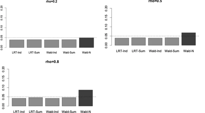
Figure 1 Type I errors in simulation set-up A withb11¼1;b1j¼0ðj6¼1Þ:n¼1000;p¼4:Wald-N denotes the GEE Wald test using individual level

(7)

wheres^2is the estimated variance of the error terms for the naive model, which assumes the error terms are identically independently distributed.

The new testing procedure includes a few steps.

1. EstimateXk9Yj;Xk19Xk2andYj19Yj2using the summary sta-tistics, reference panels, and null SNPs.

2. Obtain the OLS estimateB^v¼ ðG9Xy9XyGÞ21G9Xy9Y:

3. Estimate S^ andV^ ¼S^5In from the residuals. The

pro-cedure is the same as step 3 in the previous section. 4. Calculate the ðpqþp2₂_p_Þ₃_ð_pq_þ_p2₂_p_Þ_sandwich

co-variance matrix estimate

C¼ ðG9Xy9XyGÞ21G9ðXy9VX^ yÞGðG9Xy9XyGÞ21:

whereXy9Xy can be obtained in the same way as we did in

the previous section, andXy9VX^ y can be derived by

Xy9VX^ y ¼

! 5S:^

For the naive method, we can simply use ½n2pðqþ p21ÞS=½2n2pðqþp21Þ to estimates^2;where Sis the sum of the diagonal elements of S:^ By simple algebra, ½n2pðqþp21ÞSis indeed the sum of squared errors for the naive model.

5. The test statistics are

tj¼Bv^ 9Vj9½VjC21Vj921VjBv^ and

T1¼ min

j¼1;:::;ptj:

We reject H0 only ift0.x2pðaÞ andT1.x2p21ðaÞ:If we

want to apply the naive method instead, replace C withCnaive¼s^2ðXy9XyÞ21:

Note that this method can also be applied to the analysis adjusting for a few SNPs only, or only for a subset of traits, or their combination. We may extend the methods to sequential tests of multiple associated traits as discussed in Schaidet al. (2016) in the future.

Dealing with different samples

Sometimes the summary statistics for different traits may be based on completely different samples (i.e., no overlapping subjects). We can modify the Wald test to carry out the cor-responding pleiotropy testing. There are two possible ways.

Approach 1:Note that the OLS estimates for the joint model

of all traitsvs.SNPs are the same as OLS estimates for sepa-rate models of each traitvs.SNPs. Also, since different traits are obtained from different subjects, they are independent, meaning thatS^should be diagonal. Thejth diagonal element ofS^should simply be the estimated variance of the error term in the regression model for trait j vs. SNPs, which can be calculated by ½seðb^1jÞ

2

Xind;j9Xind;j; where Xind;j9Xind;j is the

sum of squares of X for thejth sample (the sample for getting marginal effects on traitj). We can estimateXind; j9Xind; jby

cni;assumingXind; j9Xind; jis proportional to the sample size.

(8)

Since the scale of X does not affect the result, we can simply setcto be 1.

Approach 2: Assume different samples with sample sizesnj

are obtained by a random partition of a whole sample with sample sizen¼Pnj:Build the joint model for all

P

nj

sub-jects so that we do not need to change our previous model. We can assume thatb^kjbased on allnsubjects is the same

as that based on justnjsubjects (when the sample size is large).

NowðYj9YjÞ*2ðX19X1Þ*b^1j2¼ ðnj21ÞðX19X1Þ*varcð^b1jÞ;where

ðYj9YjÞ*andðX19X1Þ*are theYj9YjandX19X1 fornjsubjects.

We can also assume Yj9Yj for all subjects is approximately

nðYj9YjÞ*=nj;X19X1 approximatelynðX19X1Þ*=nj:As a result,

we still have Yj9Yj2X19X1b^1j2 ðn21ÞX19X1varcðb^1jÞ:

Hence, we do not need to modify any formulas. We just need to inputnasPnj:

The two approaches address two different questions. Take a simple example with two traitsY1;Y2and one SNPX:Suppose

n1subjects were taken to obtain the summary statistics forY1

vs. X; and different n2 subjects were used to calculate the

summary statistics for Y2 vs. X: For the ﬁrst approach, the

alternative hypothesis is thatXis associated with the two pop-ulations, from which then1 subjects (forY1) and then2

sub-jects (forY2) were drawn respectively, allowing the two sets of

subjects to come from two, possibly different, populations. Rejecting the null hypothesis does not guarantee thatXis also associated with theﬁrst population’s second traitY2:However,

for the second approach, the alternative hypothesis is thatX inﬂuences bothY1andY2;assuming all the subjects came from

the same population. Hence, the results of the two approaches may be different if the study populations for different traits are indeed different. Nevertheless, in our opinion, the second ap-proach is preferred under the common assumption that the study populations are the same, since it can then tell whether a SNP is indeed associated with more than one trait for the same population, which follows the deﬁnition of pleiotropy. Of course, in the second approach we have to assume a common population, which may be violated in practice.

Data availability

The Cotsapas dataset can be downloaded from the online version of Cotsapaset al.(2011). The 2010 (Teslovichet al. Figure 3 Power withb11¼1;b22¼1; r¼0:3;b12¼0; n¼1000; nref¼1000;and a nominal signiﬁcance level of 0.05.

Table 4 Type I errors withn¼1000

b1 b3

Nominal signiﬁcance level = 0.05

Marginal Conditional

LRT-Ind LRT-Sum LRT-Ind LRT-Sum Wald-Ind Wald-Sum Wald-Ind-N Wald-Sum-N

0 0.3 0.042 0.041 0.041 0.041 0.040 0.041 0.040 0.040

0.6 0.042 0.041 0.041 0.041 0.040 0.041 0.040 0.040

0.9 0.042 0.041 0.041 0.041 0.040 0.041 0.040 0.040

1.2 0.042 0.041 0.041 0.041 0.040 0.041 0.040 0.040

(9)

2010) and 2013 (Willeret al.2013) lipid data are also pub-licly available athttp://csg.sph.umich.edu/abecasis/public/ lipids2010 and http://csg.sph.umich.edu/abecasis/public/ lipids2013/, respectively. The R package for our new meth-ods is publicly available at Github: https://github.com/ yangq001/Plei.

Results

Simulations for marginal analysis

To see whether the marginal analysis using summary statistics can control Type-I errors, we conducted simulations similar to those presented in Schaidet al.(2016). In the simulations, only a single SNP with minor allele frequency (MAF) 0.2 was used. The traits were generated from multivariate normal distributions. The variances of the error terms was all 1’s with an exchangeable correlation structure with correlationr:

Since our method only uses summary statistics, we also generated 1000 null SNPs with the same sample size to estimate the correlation between the traits. We centered the data, and performed a univariate association analysis. Then, we applied our method to the resulting summary statistics. To estimate the rejection rates, we used 1000 rep-lications under each setting.

Now the true model (for set-up A) is

Yj¼X1b1jþej ðj¼1; :::;pÞ;

ðe19 . . . ep9Þ9 Nð0;VÞ;and

V¼S5In;

where the diagonal elements of Sare all 1’s and the other elements arer:Theﬁtted model for marginal analysis can be simply expressed asYX1:

First, we considered the case when only one trait is asso-ciated with the SNP. According to Table 1, all methods had similar performances in terms of type I errors. The results were also close to those in Schaidet al.(2016). For conve-nience, we denote the various analysis methods as:

LRT-Ind: the original LRT of Schaidet al.(2016) with indi-vidual level data as implemented in R package“pleio.” LRT-Sum: the LRT with summary statistics.

Wald-Ind: the GEE-based Wald test with individual level data (to calculate X’X and correlations between traits).

Wald-Sum: the GEE-based Wald test with summary statis-tics; using a reference panel and some null SNPs to cal-culate X’X and correlations between traits.

Next, we considered the case when no trait is associated with the SNP (set-up B). Again, as shown in Table 2, all the methods performed similarly. They seemed to be conservative in this case, which is expected. Recall that the pleiotropy tests are like two-stage tests, and theﬁrst stage is the overall test of non-association, which should have a rejection rate of 0.05 (or 0.01) under this setting. The rejection rate of the combined tests is ,0.05 (or 0.01), since, to reject pleiotropy, both the overall test and the second-stage test must reject their respec-tive null hypothesis. As a result, all these pleiotropy tests turn out to be conservative, as shown in Schaidet al.(2016).

To compare statistical power of the various methods, we let some associated traits have a nonzero effect size of 0.25. The sample size was 500, and the number of traits was 10. As shown in Table 3, the new methods performed similarly to the original methods using individual level data.

Under theﬁrst simulation setting, we also carried out the Wald test in GEE (under the working independence model) using the naive covariance estimate, instead of the sandwich covariance estimate. As shown in Figure 1, as expected, this approach, denoted Wald-N, led to inﬂated type I errors when the error terms were strongly correlated (as the working in-dependence model did not hold). Hence, we recommend using the sandwich covariance.

The above cases included only one SNP. To be more general, we considered a simple scenario with two SNPs, both with MAF 0.2. The correlation between the SNPs is r. We generated the traits using the true model

Y1i Y2i

X1i;X2i

N

b11 b21

b12 b22

X1i X2i

;

1 r

r 1

:

After centering the simulated data, we obtained the summary statistics and conducted analysis adjusting for SNPs. For comparison, we also did an“unadjusted”marginal analysis with only SNP 1. We aimed to test for pleiotropy for SNP 1.

For the methods using only summary statistics, to estimate the correlation of the traits, we generated 1000 null SNPs and obtained their Z-scores by regressing each trait on each null SNP. In addition, we generated SNPs fornref_{subjects using MAF}

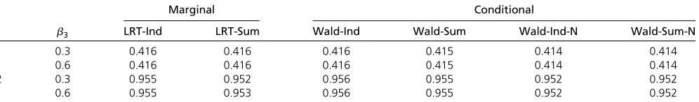
0.2 and correlationr. These were used to estimateXk19Xk2:For each replication, a new reference dataset was generated. Table 5 Power withn¼1000

b1 b3

Marginal Conditional

LRT-Ind LRT-Sum Wald-Ind Wald-Sum Wald-Ind-N Wald-Sum-N

0.1 0.3 0.416 0.416 0.416 0.415 0.414 0.414

0.6 0.416 0.416 0.416 0.415 0.414 0.414

0.2 0.3 0.955 0.952 0.956 0.955 0.952 0.952

(10)

Now theﬁtted models areYi¼b1X1iþe1ifor the

“unad-justed”marginal analysis, and areYi¼b1X1iþb2X2iþe2ifor

“adjusted”marginal analysis, where eachYincludes the two traits. We considered three versions of the Wald-Sum test:

Wald-Sum-s: using summary statistics and reference data. nref_¼_1000:

Wald-Sum-l: using summary statistics and reference data. nref_¼_10;_000:

Wald-Sum-x: using summary statistics and trueXk19Xk2:

Based on Figure 2, it appears that the unadjusted marginal analyses had the highest type I error rates. This is expected because SNP 1 is associated with trait 1, and trait 1 and trait 2 are correlated. As a result, SNP 1 is also marginally associated with trait 2, leading to that the unadjusted ginal analyses rejects the null hypothesis. Our adjusted mar-ginal analysis using summary statistics and trueXk19Xk2;Y9Y could control type I errors, but using estimates from refer-ence data resulted in inﬂated type I errors. The reason was that the estimatedXk19Xk2and the trueXk19Xk2were different. Note that Wald-Ind and Wald-Sum-x almost had the same results, suggesting that using the null SNPs to estimateY9Y was sufﬁcient.

Next, we also looked at the power of different methods. According to Figure 3, as expected, the adjusted methods were more conservative than the unadjusted methods whenb12had

the same sign asb11;since the adjusted methods could control

the type I errors. When we changed the sign ofb12;the power

of the unadjusted marginal analysis became very low, while the adjusted marginal analysis could maintain its power. Our explanation for this phenomenon is that, when two SNPs are positively correlated but have effects on the trait in different directions, their marginal effects will be diluted, so the unad-justed marginal analysis is less likely to detect pleiotropy. Note that, using the sandwich covariance and the naive covariance, matrix estimates performed similarly in the above settings, even though the two traits were correlated.

Simulations for conditional analysis

Consider a situation with one SNP and two traits. We gener-ated one SNP with MAF 0.2. The true model is

Y1i¼b1Xiþe1i;

Y2i¼b3Xiþe2i:

whereðe1i;e2iÞ’s (k¼1; 2; i¼1; 2; :::;n) are independent

normal random variables with mean 0 and variance 1 (and correlation 0).

Now the ﬁtted model for marginal analysis is Y1i¼b1Xiþe1i; Y2i¼b3Xiþe2i: For conditional analysis,

the model isY1i¼b1Xiþe1i;Y2i¼b3Xiþb2Y1iþe2i:We

ex-amined the estimated type I errors and power of marginal analysis and conditional analysis. Denote the GEE-based Wald tests by Wald-Ind-N and Wald-Sum-N after replacing the sandwich covariance matrix estimate with the naive co-variance matrix estimate.

As shown in Table 4, all the methods could control type I errors. As expected, replacing the sandwich covariance estimate by the naive covariance estimate did not really inﬂuence the result; since the error terms were uncorre-lated, the working independence model used in GEE held, leading to the good performance of the naïve covariance estimate.

As shown in Table 5, all methods gave similar power in this case. We noticed that, whenb3 .b1;increasingb3 did not

increase the power. One possible explanation is that, in this situation, the pleiotropy tests largely depend on whetherb1is

signiﬁcant. The overall test and the test for b3 are almost

always signiﬁcant, so only the test forb1 inﬂuences the

com-bined test. Whenb3is increased, the estimates ofb1and its SE

do not change much for marginal analysis, so the power does not improve. Sometimes, the estimated SE forb1may become

larger, making the test forb1 less likely to reject the null. The

extent of this is slightly greater for the conditional model. As a result, the conditional methods may even lose a little power.

In another scenario, suppose the SNP has an indirect effect on one trait through another trait. Now the model we use to simulate traits is

Y1i¼b1Xiþe1iand

Y2i¼b2Y1iþb3Xiþe2i:

whereðe1i;e2iÞ’s (k¼1; 2; i¼1; 2; :::;n) are bivariate

nor-mal random variables with variance 1 and correlation 0. They are independent of the SNP.

Again we centered the data and conducted different ways of analysis. The ﬁtted model for marginal analysis is Y1i¼b1Xiþe1i;Y2i¼b3Xiþe2i: For conditional analysis,

the model isY1i¼b1Xiþe1i;Y2i¼b3Xiþb2Y1iþe2i:

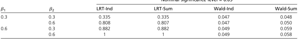
Table 6 Type I errors withn¼1000;b3¼0

b1 b2

LRT-Ind LRT-Sum Wald-Ind Wald-Sum

0.3 0.3 0.335 0.335 0.047 0.048

0.6 0.808 0.807 0.047 0.050

0.6 0.3 0.882 0.882 0.049 0.059

0.6 1 1 0.049 0.058

(11)

As shown in Table 6, the new methods could control type I errors when using individual level data, but might have slightly inﬂated type I error rates when using summary sta-tistics. In contrast, the marginal analysis could not control type I errors at all. Again, using the naive covariance or the sandwich covariance estimate did not matter in this case.

The Cotsapas data

We looked at the data offered by Cotsapaset al.(2011). The dataset contains marginal Z-scores of 107 SNPs on each of seven autoimmune diseases: celiac disease (CeD), Crohn’s disease (CD), multiple sclerosis (MS), psoriasis (Ps), rheuma-toid arthritis (RA), systemic lupus erythematosus (SLE), and type 1 diabetes (T1D). The original paper found many SNPs with pleiotropy using their proposed CPMA. For comparison, we applied various pleiotropy tests.

Note that this dataset does not contain SE, so we took the Z-scores as effect sizes and assumed the SE was 1. In addition, the summary statistics for different traits used different sam-ples, so we could apply the two approaches discussed earlier for the Wald method.

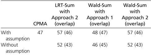
We applied different approaches to the Cotsapas data (107 SNPs, seven traits). First, we assumed we already knew that each SNP was signiﬁcant for one speciﬁc trait. Then, we tested whether more traits were associated, and compared the result with CPMA. Then, we tested pleiotropy without that assumption.

As shown in Table 7, our proposed Approach 2 detected more SNPs with pleiotropy, and covered most of the signifi -cant SNPs identified by CPMA. In this situation with marginal analysis, the Wald test and the LRT gave very similar results. When we directly applied CPMA “without assumption,” 93 SNPs became significant, which, however, were obtained because, in this case, CPMA was testing whether there was at least one association, not necessarily pleiotropy.

The lipid data

The Global Lipids Genetics Consortium GWAS study (Willer

et al.2013) has shown many loci associated with more than

one trait among LDL, HDL, TG and TC. To study this further, we conducted pleiotropy tests for single SNPs. We applied the methods to two summary association datasets based on

100,000 and 189,000 subjects, respectively (Teslovich et al.2010; Willeret al.2013), which we call the 2010 and 2013 data, respectively. The 2013 data are an expanded ver-sion of the 2010 data with more study subjects.

First, following the idea of Kimet al.(2015), we used the Z-scores of 2,371,319 nonsigniﬁcant SNPs for all traits from the 2013 data to estimate the correlations among the four types of lipids, conﬁrming their moderate to high correla-tions, which imply possible differences between marginal and conditional analyses. The results are shown in Table 8.

Next we conducted a genome-wide scan on each dataset. We tested pleiotropy for 2,363,472 SNPs that are included in both 2010 Lipids data and 2013 Lipids data. These SNPs are also present in the 1000 Genomes Project data (The 1000 Ge-nomes Project Consortiumet al.2015). We applied both mar-ginal analysis and conditional analysis. As some previous studies have shown, LDL-lowering treatments might increase the risk of type 2 diabetes partly due to their ontarget mech-anisms (Swerdlowet al.2015; Hemaniet al.2016). It might be useful to identify new drug targets by identifying genetic variants with pleiotropic effects on non-LDL lipids. To ex-clude the indirect effects of a genetic variant through LDL, we chose to conduct a conditional analysis of other lipids after adjusting for LDL. The marginal model is

LDLi¼b1Xiþe1i;

TCi¼b2Xiþe2i;

TGi¼b3Xiþe3i;and

HDLi¼b4Xiþe4i:

In contrast, the conditional model is

LDLi¼b5Xiþe5i;

TCi¼b6Xiþa6LDLiþe6i;

TGi¼b7Xiþa7LDLiþe7i;and

HDLi¼b8Xiþa8LDLiþe8i:

Note that a pleiotropic effect detected by marginal analysis could be due to indirect effect through LDL: for example, if an SNP is causal for high LDL but not for any other three traits, then, by the correlations among the traits, it will bemarginally associated with all the traits. However, with the conditional model, we can avoid such false positives; we aim to test for Table 7 Numbers of signiﬁcant SNPs (P-value<0.01)

CPMA

LRT-Sum with Approach 2

(overlap)

Wald-Sum with Approach 1

(overlap)

Wald-Sum with Approach 2

(overlap)

With assumption

47 57 (46) 48 (47) 57 (46)

Without assumption

52 (43) 46 (45) 52 (43)

“With assumption”: assuming each SNP is already known to be significant for one trait, then testing whether there is at least one more significant association;“ With-out assumption”: directly testing whether there are at least two significant associ-ations for each SNP;“Overlap”: the numbers of the significant SNPs that are also among the 47 detected ones by CPMA (“With assumption”).

Table 8 Estimated correlations between the lipid traits

TG LDL HDL TC

TG 0.228 20.414 0.324

LDL 20.087 0.873

(12)

pleiotropic effects after adjusting for LDL, which may help identify new targets for new drugs as alternatives to LDL-lowering drugs like statin. The null hypothesis for both mar-ginal and conditional pleiotropic tests is that none, or only one, ofb1;b2;b3;andb4is nonzero.

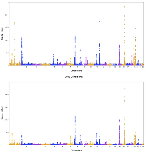
To show the difference between conditional analysis and marginal analysis, we generated some Manhattan plots. As

(13)

through LDL as an intermediate. Take SNP rs10043960 on chromosome 5 as an example. TheP-value for the pleiotropy test in marginal analysis was 9:2310210_;_{while it became}

nonsigniﬁcant at 0.74 after adjusting for LDL.

Note that if the conditional model is true, and LDLi¼

b5Xiþe5i; TCi¼0Xiþa6LDLiþe6i; which means the

SNP does not affect TC directly, then EðTCijXiÞ ¼

E½EðTCijLDLi;XiÞjXi ¼Eða6LDLijXiÞ ¼a6b5Xi: As a result,

the coefﬁcient b2 in the marginal model TCi¼b2Xiþe2i

should be b2¼a6b5: Also notice that CovðLDLi;TCiÞ ¼

CovðLDLi;a6LDLiþe6iÞ ¼a6VarðLDLiÞ;and CorðLDLi;TCiÞ ¼

a6

ffiffiffiffiffiffiffiffiffiffiffiffiffiffiffiffiffiffiffiffiffiffiffiffiffiffiffiffiffiffiffiffiffiffiffiffiffiffiffiffi

VarðLDLiÞ=VarðTCiÞ

p

:If we assume VarðLDLiÞ VarðTCiÞ;

(which may or may not hold since we do not have individual-level data to verify,) then we havea6b5CorðLDLi;TCiÞb5;

(14)

suggesting that the estimated marginal effect should be ap-proximately equal to the product of the estimated conditional effect and the correlation between the two traits. For SNP rs10043960, the marginal effect sizes on TG, LDL, HDL, and TC were 0.0096, 0.0402,20.0050, and 0.0401, respectively. If we multiply the effect size on LDL by the estimated corre-lation between LDL and each of the other traits (shown in Table 8), we get 0.0092,20.0035, and 0.0351 for TG, HDL, and TC, which are close to the estimated marginal effects. This may suggest that indirect effects through LDL can ex-plain the marginal effects of the SNP on TG, HDL, and TC.

Meanwhile, the signiﬁcance levels of some SNPs did not change, or even increased after adjusting for LDL. For SNP rs7259679 on chromosome 19, the P-value for marginal pleiotropic effects was 4:031026_; _{while the conditional}

P-value was 6:3310213_:_{The sign of the effect on LDL and}

the signs of the effects on TG and TC were opposite, while the estimated correlations between LDL, and TG and TC were positive and not small, which resembles the special case dis-cussed above (Table 5). The true effects on LDL, TG, and TC were very likely to be larger than the marginal effects. As a result, the conditional method detected pleiotropy by looking at the true effects, while the marginal method did not.

A simple (and perhaps popular) way to conduct marginal analysis is to look at the marginalP-values for each SNPvs. each trait. If a SNP has at least two significantP-values, we reject the null hypothesis of no pleiotropy. Since this ap-proach involves multiple testing across multiple traits, we apply the Bonferroni adjustment, leading to a genome-wide significance threshold of 5e28 divided by the number of traits (i.e., four here). To distinguish this from the marginal analysis described in the previous sections, called“marginal, new,” we call this univariate/single trait testing-based method“marginal, univariate.”Next, we mapped the signif-icant SNPs to loci for each analyses, following the same pro-cedure as used by Schizophrenia Working Group of the Psychiatric Genomics Consortiumet al.(2014). As shown in Figure 6, most of the loci detected by“marginal univariate” analysis were recovered by the new marginal test, while the latter found many more significant loci. The results of condi-tional analysis and marginal analysis differed, which might suggest that the effects of certain loci on some traits were indirect, with LDL as an intermediate.

Discussion

We have presented new tests for genetic pleiotropy based on either marginal analysis or conditional analysis using summary statistics. For marginal analysis with only nontrait covariates (i.e., exogenous variables), we extend and apply the LRT of Schaidet al.(2016). For conditional analysis with some traits as both responses and predictors (i.e., endogenous variables), in addition to extending the LRT of Schaidet al.(2016), for robustness, we also propose using the Wald test in GEE with the working independence model and its corresponding sand-wich covariance matrix estimate. Note that we assume a re-cursive system, for which the OLSE (i.e., GEE estimator with the working independence model) is unbiased (Hanushek and Jackson 1977, p. 229); more general structural equation mod-els (Liet al.2006; P. Wanget al.2016) may require a two-stage least squares estimator, which is much more complex and, more importantly, it is unclear whether it can be applied to summary statistics only. Our extensive simulations showed that our conditional method performed better than marginal analysis in terms of controlling type I errors when indirect effects existed. In some cases, the conditional analysis even had higher power than the marginal analysis. Marginal anal-ysis adjusting for SNPs is also better than unadjusted marginal analysis in certain cases. We applied our methods to the Cot-sapas data, and found more SNPs with genetic pleiotropy, cov-ering most of those detected by Cotsapaset al.(2011). We also applied different approaches to the 2010 and 2013 lipid data to show possible differences between marginal and condi-tional analyses.

In the future, we may extend our methods to sequential tests of multiple associated traits as discussed in Schaidet al. (2016).

Acknowledgments

We thank the editors and reviewers for many detailed and helpful comments. This research was supported by National Institutes of Health grants R01GM113250, R01HL105397, R01HL116720, and R21AG057038, and by the Minnesota Supercomputing Institute at the University of Minnesota.

Literature Cited

Berger, R. L., 1997 Likelihood ratio tests and intersection-union tests, pp. 225–237 inAdvances in Statistical Decision Theory and Applications. Birkhäuser, Boston.

Boekholdt, S. M., B. J. Arsenault, S. Mora, T. R. Pedersen, J. C. LaRosaet al., 2012 Association of LDL cholesterol, non-HDL cholesterol, and apolipoprotein B levels with risk of cardiovas-cular events among patients treated with statins: a meta-analysis. JAMA 307: 1302–1309.

Chung, D., C. Yang, C. Li, J. Gelernter, and H. Zhao, 2014 GPA: a statistical approach to prioritizing GWAS results by integrating pleiotropy and annotation. PLoS Genet. 10: e1004787. Cotsapas, C., B. F. Voight, E. Rossin, K. Lage, B. M. Neale et al.,

2011 Pervasive sharing of genetic effects in autoimmune dis-ease. PLoS Genet. 7: e1002254.

(15)

Deng, Y., and W. Pan, 2017 Conditional analysis of multiple quantitative traits based on marginal GWAS summary statistics. Genet. Epidemiol. 41: 427–436.

Do, R., C. J. Willer, E. M. Schmidt, S. Sengupta, C. Gao et al., 2013 Common variants associated with plasma triglycerides and risk for coronary artery disease. Nat. Genet. 45: 1345–1352. Hanushek, E. A., and J. E. Jackson, 1977 Statistical methods for

social scientists. New York: Academic Press.

Hemani, G., J. Zheng, K. H. Wade, C. Laurin, B. Elsworthet al.,

2016 MR-Base: a platform for systematic causal inference

across the phenome using billions of genetic associations. bioRxiv. Available at:https://www.biorxiv.org/content/early/ 2016/12/16/078972.

Kim, J., Y. Bai, and W. Pan, 2015 An adaptive association test for multiple phenotypes with GWAS summary statistics. Genet. Ep-idemiol. 39: 651–663.

Kim, J., Y. Zhang, and W. Pan Alzheimer’s Disease Neuroimaging Initiative, 2016 Powerful and adaptive testing for multi-trait and multi-SNP associations with GWAS and sequencing data. Genetics 203: 715–731.

Kwak, I., and W. Pan, 2016 Adaptive gene- and pathway-trait

association testing with GWAS summary statistics. Bioinfor-matics 32: 1178–1184.

Kwak, I., and W. Pan, 2017 Gene- and pathway-based association tests for multiple traits with GWAS summary statistics. Bioinfor-matics 33: 64–71.

Li, C., C. Yang, J. Gelernter, and H. Zhao, 2014 Improving genetic risk prediction by leveraging pleiotropy. Hum. Genet. 133: 639–650. Li, R., S.-W. Tsaih, K. Shockley, I. M. Stylianou, J. Wergedalet al.,

2006 Structural model analysis of multiple quantitative traits. PLoS Genet. 2: e114.

Majumdar, A., T. Haldar, and J. S. Witte, 2016 Determining which phenotypes underlie a pleiotropic signal. Genet. Epidemiol. 40(5): 366–81.

Sampson, U. K., S. Fazio, and M. F. Linton, 2012 Residual cardio-vascular risk despite optimal LDL cholesterol reduction with statins: the evidence, etiology, and therapeutic challenges. Curr. Atheroscler. Rep. 14: 1–10.

Schaid, D. J., X. Tong, B. Larrabee, R. B. Kennedy, G. A. Poland et al., 2016 Statistical methods for testing genetic pleiotropy. Genetics 204: 483–497.

Schizophrenia Working Group of the Psychiatric Genomics Consor-tium, 2014 Biological insights from 108 schizophrenia-associated genetic loci. Nature 511: 421–427.

Solovieff, N., C. Cotsapas, P. H. Lee, S. M. Purcell, and J. W. Smol-ler, 2013 Pleiotropy in complex traits: challenges and strate-gies. Nat. Rev. Genet. 14: 483–495.

Stephens, M., 2013 A uniﬁed framework for association analysis with multiple related phenotypes. PLoS ONE 8(7): e65245. Available at:https://doi.org/10.1371/journal.pone.0065245. Swerdlow, D. I., D. Preiss, K. B. Kuchenbaecker, M. V. Holmes, J. E.

Engmannet al., 2015 HMG-coenzyme A reductase inhibition, type 2 diabetes, and bodyweight: evidence from genetic analysis and randomised trials. Lancet 385: 351–361.

Teslovich, T. M., K. Musunuru, A. V. Smith, A. C. Edmondson, I. M. Stylianouet al., 2010 Biological, clinical and population rele-vance of 95 loci for blood lipids. Nature 466: 707–713. The 1000 Genomes Project ConsortiumAuton, A., L. D. Brooks,

R. M. Durbin, E. P. Garrisonet al., 2015 A global reference for human genetic variation. Nature 526: 68–74.

Toth, P. P., 2016 Triglyceride-rich lipoproteins as a causal factor for cardiovascular disease. Vasc. Health Risk Manag. 12: 171– 183.

Wang, P., M. Rahman, L. Jin, and M. Xiong, 2016 A new statisti-cal framework for genetic pleiotropic analysis of high dimen-sional phenotype data. BMC Genomics 17: 881.

Wang, Q., C. Yang, J. Gelernter, and H. Zhao, 2015 Pervasive pleiotropy between psychiatric disorders and immune disorders revealed by integrative analysis of multiple GWAS. Hum. Genet. 134: 1195–1209.

Wang, Y., A. Liu, J. L. Mills, M. Boehnke, A. F. Wilson et al., 2015 Pleiotropy analysis of quantitative traits at gene level by multivariate functional linear models. Genet. Epidemiol. 39: 259_–275.

Wang, Z., Q. Sha, and S. Zhang, 2016 Joint analysis of multiple traits using_“optimal_”maximum heritability test. PLoS One 11: e0150975.

Willer, C. J., E. M. Schmidt, S. Sengupta, G. M. Peloso, S. Gustafsson et al., 2013 Discovery and re_ﬁnement of loci associated with lipid levels. Nat. Genet. 45: 1274_–1283.