Three Unit Series–Parallel Systems with
Common Cause and Environmental Error
Failures by Probabilistic Analysis
K. Uma Maheswari1, A. Mallikarjuna Reddy2
Department of Mathematics, Shri Shirdi Sai Institute of Science & Engineering, Vadyampeta, Anantapuramu, (A.P.),
India1,2
ABSTRACT: In this paper it is proposed for three unit series parallel system the nature of reliability proposed a better model for common cause and environmental error failures by three unit series parallel system. We consider three models of a three unit series parallel system consisting of the units A, B and C which is in function state. When A is functioning and either B or C are in functioning state and we assume that the system is subjected to common cause and environmental error failures.
KEYWORDS:Series-parallel system, common cause, Environmental error, Gamma distribution, Availability
I. INTRODUCTION
In reality the systems under consideration may not be modelled as series or parallel systems. If the functional diagram suggests that the successful operation of the systems depends on the proper operation then we say that the system configuration is a series. A system with ‘m’ components is known as m-unit parallel system if and only if the successful functioning of any one of the components leads for the system success. In this chapter we consider a three unit series parallel system and we study the reliability and availability analysis of the system is subjected to common cause and environmental error failures.
II. ASSUMPTIONSANDNOTATION
We consider three models of a three unit series-parallel system consisting of the units A, B and C which is in functioning state only, when A is functioning and either B or C are in functioning state, and we assume that the system is subjected to common-cause and environmental error failures.
ASSUMPTIONS
At any time epoch‘t’ the system can be in one of the following seven states.
0 The state of the system with all the three components functioning state.
1 The state of the system with the component A and one of the components B or C is in functioning state.
2 The failed state of the system corresponding to the failure A from the state ‘0’. 3 The failed state of the system due to the failure of the component A from state 1.
4 The failure state of the system corresponding to the failure of both the components B and C while A is functioning.
NOTATION
T = Time
S = Laplace transform variable
= Constant failure rate of the units A and B
Cl = Constant common cause failure rate of the system from the state ‘0’.
e = Constant environmental error failure rate of the system
C2 = Constant common cause failure rate of the system from state 1.
A = Constant failure rate of the unit A.
= Constant repair rate of a unit.
1 = Constant repair rate of the system from the state 4.
2 = Constant repair rate of the system from the failed state 3.
Pk(x,t) = Probability density (with respect to repair time) that the failed system is in state k and has an elapsed repair time of x, for k = 5, 6.
k (x), qk (x) = Repair rate and probability density function of repair time respectively when the failed system is in state k and has an elapsed repair time of x, for k = 5, 6.
= The shape parameter of the Gamma probability density function.
III. ANALYSIS
CASE – I: With the above notation the transition diagram of the system is given by The system of integral differential equations associated with this model are given by
0
0
( )
(2
cl e A)
( )
dp t
p t
dt
p t
1( )
Ap t
2( )
1p t
4( )
2p t
3( )
5 5 6 6
0 0
( , )
( )
( , )
( )
p x t
x dx
p x t
x dx
(1)1
2 1 0
( )
(
A C)
( )
2
( )
dp t
p t
p t
dt
(2)2
2 0
( )
( )
( )
A A
dp t
p t
p t
dt
(3)3
2 3 1
( )
( )
A( )
dp t
p t
p t
dt
(4)4
1 4 1
( )
( )
A( )
dp t
p t
p t
dt
(5)5
( )
x
p x t
5( , )
0
x
t
(6)
6
( )
x
p x t
6( , )
0
x
t
(7)The initial conditions are given by
P0 (0) = 1 and pj (0) = 0 for j = 1, 2, 3, 4 Pk (x,0) = 0 for k = 5, 6
By taking Laplace Transformations the above equations reduces to
s p0 (s) – 1 + (2 + cl + e + A) p0 (s) = p1 (s) + = A p2 (s) + = 1 p4 (s) + 2 p3 (s)
+ 5 5 6 6
0 0
( , )
( )
( , )
( )
p x s
x dx
p x s
x dx
(10)s p1 (s) + ( + c2 + + A) p1 (s) = 2 p0 (s) (11)
s p2 (s) + A p2 (s) = A p0 (s) (12)
s p3 (s) + 2 p3 (s) = A p1 (s) (13)
s p4 (s) + 1 p4 (s) = p1 (s) (14)
5
( )
5( , )
0
s
x
p x s
x
(15)0
( )
6( , )
0
s
x
p x s
x
(16)p5 (0, s) = e p0 (s) (17)
p6 (0, s) = c1 p0 (s) + c2 p1 (s) (18) From equations (11) to (14)
0 1
2
2
( )
( )
A c
p s
p s
s
2
( )
0( )
A
A
p s
p s
s
3 1 0
2 2
2
( )
( )
( )
(
) (
)
A A
A A c
p s
p s
p s
s
s
s
2
4 1 0
1 1 2
2
( )
( )
( )
(
) (
A c)
p s
p s
p s
s
s
s
0 1 0 0 2
2
( ) 1 (2
c e A)
( )
( )
A c
s p s
p s
p s
s
2 1 0 0 1 22
( )
( )
(
) (
)
A AA A c
p s
p s
s
s
s
2 0 2 22
( )
(
) (
)
A A cp s
s
s
5 5 6 6
0 0
( , )
( )
( , )
( )
p x s
x dx
p x s
x dx
From equation (15)
5
( , )
(
5( ))
5( , )
p x s
s
x p x s
x
5 5 5( , )
(
( ))
( , )
p x s
x
s
x
p x s
Integrating we obtain
5 0 5
0
(log
( , ))
( )
x x
p x s
sx
x dx
5
5
5 0
log
( , )
( )
(0, )
x
p x s
sx
x dx
p
s
5 0 ( ) 5 5
( , )
(0, )
x sx x dxp x s
e
p
s
5 0 ( )5
( , )
5(0, )
x sx x dx
p x s
p
s e
5 0 ( )0
( )
x sx x dx
e
e
p s
Again from equation (16) we have (19)
6 0
( )
6
( , )
6(0, )
x sx x dx
p x s
p
s e
5 0 ( ) 2 1 0 22
( )
x sx x dx cc
A c
p s e
s
(20)From equation (10) we have
2 1
0 1 0 0 0 0
1 2 1 3
2
2
( ) 1 (2
)
( )
( )
( )
( )
(
) (
)
A A
c e A
s p s
p s
p s
p s
p s
s
A
s
A
s
A
s
A
5 0
( ) 2
0 5 0
1 4 0
2
( )
( )
( )
(
) (
)
sx x dx A
h
p s
e
x dx p s
s
A
s
A
6 0 ( ) 21 0 6
1 0
2
( )
( )
(
)
x sx x dx cc
p s e
x dx
s
A
On simplification we obtain
1 2 3 4
0
((
) (
) (
) (
))
( )
( )
s
A
s
A
s
A
s
A
p s
Q s
(21)SPECIAL CASE MODELS - AVAILABILITY
As a special case we assume that the repair time distribution of the failed system will follow Gamma distribution with shape parameter In this case one has
5 1
5 5
5
(
)
( )
;
0,
0
( )
x
x
e
q x
t
(22)and 6 1 6 6 6
(
)
( )
;
0,
0
( )
x
x
e
q x
t
(23)(1) We assume that the shape parameter =1. In this case the repair of the failed system is constant and its repair times are exponentially distributed. Hence we
5
5
( )
5x
q x
e
(24)and 6
6
( )
6x
q x
e
(25)Taking Laplace transform we obtain
5 6
5 6
5 6
( )
( )
q s
and q s
s
s
(26)substituting these results into equation (21) one obtain
0 0 0
( )
( )
( )
N s
p s
s D s
where
N0(S) = S6 + B1S5 + B2S4 +B3S3 + B4S2 + B5S + B6 D0(S) = S6 + B7S5 + B8S4 +B9S3 + B10S2 + B11S + B12
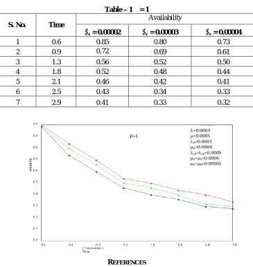
The time dependent system availability AV(t) for this system is given by AV(t) = P0(t) + P1(t)
= (G1 + G8) + (G2 + G9) es1t + (G3 + G10) es2t + (G4 + G11) es3t (G5 + G12) es4t + (G6 + G13) es5t + (G7 + G14) es6t
Limiting availability (steady state) AV of the system is given by
1 8
( )
( )
V V
t
A t
Lt A t
G
G
Table – 1 = 1 S. No. Time
Availability
e = 0.00002 e = 0.00003 e = 0.00004
1 0.6 0.85 0.80 0.73
2 0.9 0.72 0.69 0.61
3 1.3 0.56 0.52 0.50
4 1.8 0.52 0.48 0.44
5 2.1 0.46 0.42 0.41
6 2.5 0.43 0.34 0.33
7 2.9 0.41 0.33 0.32
REFERENCES
1. M Dhilon, B.S and O.C Anude: Commona cause failure analysis of a parallel system with warm stand by, Micro-Electronics and Reliability –
Vol.33, No.9, PP.1321-1342, (1993).
2. Dhillon, B.S and Yan, N. : Reliability and Availability analysis of warm stand by systems with common-cause failures and human errors. Micro