ABSTRACT
VEREEN, STEPHANIE CAROL. Forecasting Skilled Labor Demand in the US Construction Industry. (Under the direction of Dr. William Rasdorf and Dr. Joseph Hummer.)
Ensuring an adequate supply of skilled laborers to meet demand and avoid potential shortages or surpluses has been an issue of concern to construction industry professionals and researchers for quite some time. Poor industry image, declining wages, lack of training opportunities, and training time lag between new, unskilled laborers becoming skilled are a few of the many factors identified by researchers and professionals over the past 20 years as having contributed to skilled labor mismatch. Although construction unemployment reached record high levels in February of 2007 (27.1%) due to poor economic conditions in the United States, as we continue through the 2010‟s and into the 2020‟s, maintaining an adequate and competitive workforce that is able to meet the future skilled labor demands is an issue of importance to the construction industry.
Forecasts of skilled construction labor demand provide valuable information that can ensure that construction industry participants and stakeholders are aware of future labor force needs and are prepared to recruit, train, and retain an adequate pipeline of skilled laborers. Forecasts of skilled labor demand for the construction industry are important to ensuring a sustainable skilled labor workforce. Therefore, the main objective of this work was to make accurate and useful forecasts of future skilled construction labor demand.
Crucial to developing reliable forecasts is the collection of accurate and consistent data with which models can be developed and on which to base projections. Data were collected in this effort for five key independent variables (interest rate, material price, construction output, productivity, and real wage) and the dependent variable (labor demand) from a variety of existing data sources. The availability and quality of economic and construction industry data intended for use in the skilled labor demand forecast model is assessed and evaluated.
construction activities in the RS Means Building Construction Cost Data manual. The newly developed metric was used as input to the developed forecast model.
The model developed in this research used vector autoregression (VAR). VAR modeling was selected because of its ability to analyze multivariate time series data. The forecast model was successfully validated against two years of actual data.
Potential data trends for each independent model variable were developed. Various combinations of the potential trends were used in the model to formulate and compare different forecast scenarios through 2023. The most likely scenario results in a forecasted need of approximately 5.3 – 6.3 million skilled laborers needed in the construction industry by 2023.
Recommendations are given as to how the availability and quality of construction industry labor data can be improved. One key recommendation is that more extensive data collection can be undertaken to produce accurate and consistent data. Doing so will provide support for more accurate forecasts for planning, recruitment, and retention efforts. Also, the industry should use and strive to improve the newly developed metric for construction industry labor productivity, since this allows construction professionals to be able to analyze industry level productivity by means of a commonly used industry reference manual.
Forecasting Skilled Labor Demand in the US Construction Industry
by
Stephanie Carol Vereen
A dissertation submitted to the Graduate Faculty of North Carolina State University
in partial fulfillment of the requirements for the Degree of
Doctor of Philosophy
Civil Engineering
Raleigh, North Carolina 2013
APPROVED BY:
_________________________________ _________________________________
Dr. Edward Jaselskis Dr. Walter Wessels
_________________________________ _________________________________
Dr. William Rasdorf Dr. Joseph E. Hummer
ii
DEDICATION
iii
BIOGRAPHY
iv
ACKNOWLEDGEMENTS
I would like to express a special gratitude to Dr. Joseph Hummer and Dr. William Rasdorf. Their professional and personal guidance and support of my graduate studies made this dissertation possible. I would also like to thank Dr. Edward Jaselskis and Dr. Walter Wessels for the advice and support provided as members of my advisory committee. I look forward to future collaborations.
I would also like to thank the faculty and staff of the North Carolina State University Department of Civil, Construction, and Environmental Engineering. Many of you have provided constant support and encouragement during my graduate school experience. I would like to thank Zhongkai Liu, Shikai Luo, and Dr. Peter Bloomfield of NCSU Statistics for their support of this project.
I would like to acknowledge the financial support I have received for my graduate studies from the North Carolina State University Minority Engineering Programs/National Science Foundation, the North Carolina State University Graduate School, and the Conference of Minority Transportation Officials (COMTO).
v
TABLE OF CONTENTS
LIST OF TABLES ... ix
LIST OF FIGURES... x
1.0 INTRODUCTION ... 1
1.1 Research Objectives ... 2
1.2 Scope ... 4
1.3 Outcomes and Benefits ... 5
2.0 DATA COLLECTION OPPORTUNITIES AND CHALLENGES ... 7
2.1 Background ... 8
2.2 Scope ... 9
2.3 Data Quality ... 11
2.4 Previous Work ... 12
2.5 Data Collection Sources and Challenges ... 14
2.5.1 Labor Demand ... 15
2.5.2 Interest Rate ... 19
2.5.3 Material Price ... 20
2.5.4 Construction Output ... 21
2.5.5 Construction Spending ... 23
2.5.6 Productivity ... 30
2.5.7 Real Wage ... 32
2.6 Conclusions ... 32
2.7 Recommendations ... 34
3.0 DEVELOPMENT AND COMPARATITVE ANALYSIS OF CONSTRUCTION INDUSTRY LABOR PRODUCTIVITY METRICS ... 35
vi
3.2 Scope ... 37
3.3 Defining and Measuring Construction Industry Labor Productivity ... 37
3.3.1 Definition of Construction Industry Labor Productivity ... 38
3.3.2 Measurement of Construction Productivity ... 38
3.3.3 BLS Multifactor Productivity Index for Construction ... 39
3.4 Literature Review ... 41
3.4.1 Literature That Used RS Means ... 42
3.5 Development of a CILP Metric Using RS Means ... 45
3.5.1 About RS Means Data... 45
3.5.2 Data Collection from RS Means ... 47
3.5.3 Metric Development ... 51
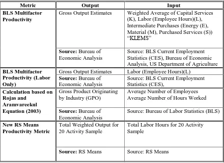
3.6 Comparison of RS Means Based CILP Metric to Existing Metrics ... 52
3.6.1 BLS MFP Data ... 52
3.6.2 Rojas and Aramvareekul ... 54
3.7 Comparison and Analysis of All Metrics ... 57
3.8 Conclusions and Recommendations ... 59
4.0 DEVELOPMENT OF A VECTOR AUTOREGRESSION MODEL TO FORECAST SKILLED LABOR DEMAND ... 62
4.1 Research Objectives ... 64
4.2 Scope ... 65
4.3 Literature Review ... 67
4.4 Data Collection and Transformation ... 71
4.4.1 Labor Demand and the Independent Variables... 72
4.4.2 Data Transformations ... 75
vii
4.5.1 Vector Autoregression ... 81
4.5.2 Model Specification ... 83
4.5.3 Forecast Trials ... 83
4.5.4 Diagnostic Tests ... 89
4.6 Conclusions ... 90
5.0 APPLICATION AND RESULTS OF THE MODEL ... 93
5.1 Objective ... 94
5.2 Literature Review ... 95
5.3 Methodology ... 98
5.3.1 The Model ... 98
5.4 Potential Trends for the Independent Variables ... 100
5.4.1 Material Price ... 101
5.4.2 Productivity ... 102
5.4.3 Real Wage ... 103
5.4.4 Construction Output ... 104
5.5 Forecast Scenario and Results ... 106
5.5.1 Each Variable Examined Independently ... 106
5.5.2 All Variables Trend at the Same Magnitude ... 107
5.5.3 Independent Variable Behaves Differently than Historically ... 108
5.5.4 Extreme Value Analysis ... 110
5.5.5 Overall Analysis ... 112
5.6 Conclusions ... 113
5.7 Recommendations ... 114
REFERENCES ... 116
viii
A. Evaluation of Construction Industry Occupations ... 128
B. RS Means Activity ID... 135
C. Productivity Data Final Sample... 137
D. Other Independent Variables ... 160
E. Data Sets ... 166
F. Unit Root Test Results ... 173
ix
LIST OF TABLES
Table 2.1. Evaluation of Data Sources for Labor Demand ... 15
Table 2.2. Sample Derivation of Monthly Square Footage of Construction Using USCB and RS Means Data for January 2010 ... 27
Table 2.3. Comparison of USCB Public Construction Category Changes, January 1990 vs. January 1993 ... 29
Table 3.1. Common Measures of Labor Productivity ... 38
Table 3.2. Outcome of Productivity Analysis in Other Literature ... 44
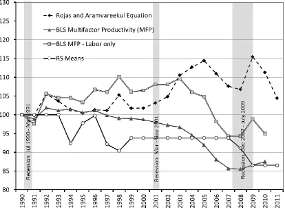
Table 3.3. Sample RS Means Activity ... 46
Table 3.4. Sample Set of RS Means Construction Activities ... 49
Table 3.5. Data Sources for Each Productivity Metric ... 57
Table 4.1. Summary of AIC and BIC Analysis ... 85
Table 4.2. MAPE and Theil‟s U Value for Selected Trials ... 86
Table 5.1. Possible Extreme Values of Labor Demand in the Future ... 111
Table B.1. RS Means Activity ID‟s – Changes Over the Years ... 136
Table C.1. Productivity Data Final Sample ... 137
Table D.1. Summary of Other Variables ... 161
Table D.2. R2 Values of Other Variables ... 165
Table E.1 Data Set – Labor Demand and Independent Variables, 1990 – 2011 ... 166
x
LIST OF FIGURES
Figure 2.1. Comparison of OES and CES Number of Persons Employed ... 18
Figure 2.2. BLS Producer Price Index vs. ENR Material Price Index ... 21
Figure 2.3. Labor Demand and Construction Output ... 22
Figure 2.4. USCB Construction Spending - Old and New Classification System Comparison ... 25
Figure 2.5. Comparison of Public and Private Construction Spending Totals ... 28
Figure 3.1. BLS Multifactor Productivity (MFP) for Construction Industry (NAICS 23) ... 40
Figure 3.2. Labor Productivity Graph from Rojas and Aramvareekul (2003) ... 42
Figure 3.3. Construction Industry Labor Productivity ... 51
Figure 3.4. Labor Productivity Metric Calculated from BLS MFP Data ... 53
Figure 3.5. GPO (Output) and Aggregate Weekly Hours (Input) Data ... 55
Figure 3.6. Labor Productivity Metric Calculated Using Rojas and Aramvareekul (2003) ... 56
Figure 3.7. Annual Percent Change of Each Productivity Metric ... 58
Figure 4.1. Historical Labor Demand in the U.S. Construction Industry, 1990 – 2011 [Source: BLS Current Employment Statistics] ... 73
Figure 4.2. Autocorrelation Function (ACF) Plots for Construction Output: Original (a), First Differenced (b), and Second Differenced (c) ... 77
Figure 4.3. Forecast Results for Trials 9, 15, and 17 and Actual Labor Demand ... 88
Figure 5.1. Material Price Index Historical Data (1990 – 2011) and Potential Trends (2012 – 2022) ... 101
Figure 5.2. Productivity Index Historical Data (1990 – 2011) and Potential trends (2012 – 2022) .. 102
Figure 5.3. Real Wage Historical Data (1990 – 2011) and Potential Trends (2012 – 2022) ... 103
Figure 5.4. Monthly Construction Output Data (1990 – 2011) ... 104
Figure 5.5. Construction Output Historical Data (1990 – 2011) and Potential Trends (2012 – 2022) for January and August... 105
Figure 5.6. Category 1 Labor Demand Forecast Scenarios ... 107
Figure 5.7. Category 2 Forecast Scenarios ... 108
Figure 5.8. Labor Demand Forecast Scenario Using Alternate Potential Trend for Material Price.. 109
1
1.0 INTRODUCTION
Construction is one of the largest industries in the United States. Past industry employment levels have surpassed 7.5 million workers, although as of June 2013, industry employment was about 5.8 million [BLS 2013A]. In addition to the significant portion of the population that relies on the construction industry for employment, most of the remaining population relies on the construction industry for the erection of basic infrastructure and services such as water and sewer systems, transportation systems, and hospitals.
Ensuring an adequate supply of skilled laborers to meet demand and avoid potential shortages or surpluses has been an issue of concern to construction industry professionals and researchers for quite some time. Poor industry image, declining wages, lack of training opportunities, and training time lag between new, unskilled laborers becoming skilled, are a few of the many factors identified by researchers and professionals over the past 20 years as having contributed to skilled labor mismatch [CURT 2004].
It is important to distinguish that there is not a lack of persons, or physical bodies, available to do the work. The critical issue regarding construction labor demand is skill. “A skilled craftsperson is easily identified by their reliance on their mechanical skills and their emphasis on production” [Chini 1999]. Skilled labor jobs are manual jobs that require specialized education or training. There are plenty of people to perform non-skilled construction activities, such as general help, or those that require minimal to no training and instruction. However, trades such as carpenter, electricians, and pipefitters require extensive apprenticeship or other training programs, which can take years to complete. It is not possible to simply round up unemployed, unskilled, or low skilled laborers and expect them to fill the anticipated void overnight.
2
in October 2006 [BLS 2013A]. Attention to fluctuations in skilled construction labor demand is equally important in periods of high unemployment (labor surplus), as it is during periods of low unemployment (labor shortages). “Mismatches between [labor] demand and supply in the market [cause] serious effects on the development of the industry and its ability to sustain the skilled workforce” [Wong et al 2006]. The construction industry is a dynamic operation with workers constantly circulating in and out, sometimes underserved and other times overflowing.
As of 2013, the downturn in the U.S. economy and record high unemployment rates have greatly diminished interest in modeling labor trends and identifying solutions that ensure a consistent supply of skilled workers. However, there is a still a need for research attention to skilled labor trends in the construction industry; a serious mismatch of skilled labor supply and demand resulting in critical industry shortages or surpluses is still possible.
“With the reduced need for craft labor during the economic downturn, many workers will leave construction for other industries – often permanently. Also, during slow times, fewer younger workers will begin apprenticeship or community college programs that would train them to be skilled craft workers. When the economy rebounds and the demand for construction craft labor increases again, the craft labor pool will have contracted even more and the shortage of skilled laborers will be even greater” [Skipper et al 2009].
Not enough industry action, in terms of acknowledgement, recruitment, and training, has been done to successfully generate solutions to the issue of potential skill mismatch. Additional research and recommendations are needed to result in a corrective shift in the construction industry that avoids repercussions of extreme labor shortages or surpluses.
Labor forecasting is essential to and must be incorporated into the decision making and planning processes in the construction industry. As we continue through the 10‟s and into the 20‟s, maintaining a “competitive and adequate workforce able to meet the future demands of the industry” is an issue of importance to the construction industry [Wong et al 2006].
1.1 Research Objectives
3
skilled construction labor demand in the United States. Various model outcomes will be used to analyze future skilled labor trends.
Other researchers have previously presented data and models related to skilled construction labor demand. Databases have been developed to identify long term labor supply needs [CII 1989] and existing and impending skilled labor shortages have been reported. There has been some research done on factors leading to skilled labor shortages and overages, best practices for recruiting and retaining workers, and some skilled labor demand models for other countries (Hong Kong/HKSAR, Israel, and United Kingdom). Some research was based on industry surveys, and other forecasts are proprietary in nature. The research proposed herein seeks to present a forecast demand model of skilled construction labor in the United States that incorporates multiple factors (industry-based, economics-based, etc.), which has previously not been done.
To meet the research objective, the set of tasks listed below was identified and executed:
1. Prepare a literature review about skilled labor shortages and overages, identifying and assessing research on skilled labor forecasting models and methods.
2. Identify and define factors identified as contributing to skilled labor mismatches in the construction industry.
3. Identify and classify modeling methods best suited for skilled labor forecasting and evaluate previous uses and applications of the most promising models.
4. Select a forecast modeling method. 5. Gather complete data sets.
6. Populate and exercise the selected forecast model, using collected data. 7. Revise and adjust model to achieve best fit.
8. Compare forecast model outputs with actual data to determine accuracy and effectiveness of the selected modeling method (validation).
9. Using most significant variables, forecast future construction labor demand.
10. Draw conclusions; based on forecast results, make policy and industry recommendation for addressing future construction skilled labor demand.
4
1.2 Scope
The focus of this research was mainly on skilled laborers in the U.S. construction industry. For the purpose of this research, skilled labor demand is considered to be the number of skilled craft workers needed to work on active construction projects. It could also be considered the number of skilled craft workers needed to keep these projects on schedule and on budget.
The focus on skill refers to manual jobs that require specialized training or skill. “These people typically have some type of formal training in their respective crafts and have been working in the field for many years” as opposed to a non-skilled worker who may be employed in a labor intensive occupation that requires no training or experience [Chini et al 1999]. Also, this distinction is made to delineate skilled labor in the construction industry from skilled workers in other industries.
The Bureau of Labor Statistics (BLS) publishes labor data by occupation and industry. There are 19 occupations recognized by the BLS in the construction industry; the research attempted to focus on workers in one of more of these occupation classifications. A detailed analysis of the 19 occupations was completed to determine if each occupation did indeed classify as skilled. Appendix A contains the results of this analysis which resulted in 17 or the 19 occupations identified as skilled based on job description, education, and training requirements. The data collection process revealed that it was not always possible to select data categorized specifically by the 17 occupations, so applicable designations for different data sources were selected to maintain this scope characteristic.
Data for the entire United States was used versus local or regional level data. Construction workers frequently travel and temporarily reside at a project site other than their established home area; evaluating data for all of the United States will capture demand for all workers, regardless of project or home locations. Focusing on a national demand forecast will help national trade organizations and the U.S. Congress improve the entire industry, not just a specific region, state, or city.
5
1.3 Outcomes and Benefits
Forecasting skilled construction labor demand will assist the construction industry with its ability and preparedness to train and supply an adequate pipeline of skilled laborers and will ensure a consistent and quality construction labor force. Forecasting supports planning activities and can inform the construction industry of what people are needed, when, and in what quantities.
The forecast model and potential labor demand outcomes will be useful to a variety of construction industry stakeholders. Construction business owners will have a better understanding of future staffing needs. Model outputs can assist trade and apprenticeship groups with recruitment efforts and planning for future training needs. Also, the research can provide policy advocates and makers with data to make sound decisions regarding funding and support for skilled labor needs for the United States. High demand forecasts will enable industry stakeholders to ensure that training program enrollment and completion is on track to supply the forecasted demand; or such forecasts could help a company plan project start and finish dates and plan and allocate their skilled labor resources. Correspondingly, low demand forecasts may also prompt the industry to plan; lobbying groups may work to garner government funding and support of new construction projects. Overall, effective demand forecasting can help the industry recognize labor trends and patterns which can improve planning and allocation of labor resources.
Target demand numbers forecasted using the developed model can be used by companies and professional industry organizations as a metric against which to compare the goals, objectives, and success of a variety of training, recruitment, and retention programs. Also, when a government is able to reasonably forecast future changes and demands in labor markets, they can better assist students and training programs with planning needs [Willems 1998].
6
7
2.0 DATA COLLECTION OPPORTUNITIES AND CHALLENGES
Forecasting skilled construction labor demand is useful for a variety of reasons. Forecasting supports planning activities and can inform the construction industry of which trades people are needed in, when, and in what quantities. High demand forecasts will enable construction companies and industry groups to ensure that training program enrollment and completion is on track to supply the labor to meet the forecasted demand. Correspondingly, low demand forecasts may also prompt the industry to act. For example, lobbying groups may work to garner government funding and support of new construction projects to promote skilled labor employment and income growth. “Construction employers may be able to increase the pressure on national governments to invest in the most appropriate form of skilled [labor] provision once they have a complete understanding of the [labor] resource issues affecting the construction industry” [Agapiou et al 1995a]. Effective demand forecasting can help the construction industry recognize labor trends and patterns which can improve both planning and allocation of labor resources.
Crucial to developing reliable and meaningful forecasts is the identification and collection of accurate and consistent data to use as model inputs, to base projections on, and to produce statistically relevant results. As part of the process of developing a skilled labor demand forecast model, the authors set out to identify and quantify independent variables that affect skilled labor demand. During the data identification and collection process, numerous challenges were encountered regarding the accuracy and consistency of the desired data. These are reported herein.
8
The authors seek to achieve the following objectives in this paper:
Describe efforts to collect quality data for five preliminary variables and an independent variable to be used in a construction labor demand forecast model.
Describe general and specific challenges encountered during the data collection process. Provide recommendations for achieving improved data quality and more consistent data
collection practices for the US construction industry.
The results from the presentation of these data collection efforts will improve future efforts and reduce the amount of time needed to collect data for a variety of construction industry needs. The data collection efforts presented here represent a significant effort to identify various sources and to evaluate the best ones for use in the model. Other researchers and industry professionals seeking labor data can benefit from this effort. Also included are recommendations for the improvement of data collection efforts by the construction industry community (researchers, contractors, owners, government agencies) that will ultimately provide improved resources for future studies, forecasts, and project planning efforts.
2.1 Background
Labor forecasting must be incorporated into the decision making and planning processes of the construction industry in the policy, academic, professional, and governmental arenas. Forecasting skilled construction labor demand ensures that the construction industry is able to have a balanced pipeline of skilled laborers available and ensures that the availability of the right labor is achieved. “A key aspect is to try to develop an understanding of the main casual factors influencing the demand for construction skills” [Briscoe and Wilson 1993]. Early in our work on construction labor demand forecasting, five variables were identified as being crucial to forecasting skilled labor demand:
9
These variables were first identified by Wong, Chan, and Chiang [2007] and were used in several models to forecast construction labor demand in Hong Kong. One or more of the variables were also used by a number of other labor demand researchers in the construction industry [Uwakweh and Maloney 1991; Briscoe and Wilson 1993; Rosenfeld and Warszawski 1993]. Most of this previous research was performed outside the US. The forecasting model that is discussed in this paper focused on skilled construction workers employed in the US construction industry.
2.2 Scope
The data addressed herein focuses on skilled construction laborers in the US construction industry and can be characterized as follows.
US construction industry – Industries are classified by the BLS using the North American Industry Classification System (NAICS). The construction industry identifier is NAICS Sector 23, Construction.
Construction laborers – The Federal government uses the Standard Occupational Classification (SOC) to organize workers and jobs into categories. Construction occupations are primarily located in Section 47, Construction and Extraction Occupations.
Skilled labor – The BLS Occupational Outlook Handbook lists 19 trades related to construction. Each of the 19 trades falls under SOC 47. The 19 trades and their specific SOC designations follow.
o Boilermakers (47-2010)
o Brickmasons, blockmasons, and stonemasons (47-2020) o Carpenters (47-2030)
o Carpet, floor, and tile installers and finishers (47-2040)
o Cement masons, concrete finishers, and terrazzo workers (47-2050) o Construction laborers (47-2060)
o Construction equipment operators (47-2070)
o Drywall and ceiling tile installers, tapers; Plasterers, and stucco masons (47-2080, 47-2160)
o Electricians (47-2110) o Glaziers (47-2120)
10 o Painters and paperhangers (47-2140)
o Plumbers, pipelayers, pipefitters, and steamfitters (47-2150) o Roofers (47-2180)
o Sheet metal workers (47-2210)
o Structural and reinforcing iron and metal workers (47-2220, 47-2170) o Construction and building inspectors (47-4010)
o Elevator installers and repairers (47-4020) o Hazardous materials removal workers (47-4040)
Skilled laborers are considered to be workers that “have some type of formal training in their respective crafts” [Chini et al 1999]. The authors used the BLS Occupational Outlook Handbook (OOH) to analyze each of the 19 BLS occupations identified above to determine the level of training and skill attainment required for each. The types of training included apprenticeship, informal training, formal education (technical college, vocational school, trades school, community college, etc.), industry based training, on the job training, supplemental classroom instruction, and combinations of any of these. The analysis concluded that 17 of the 19 occupations were skilled occupations based on training requirements. The OOH did not indicate any specific training requirements for Construction and building inspector (47-4010) and hazardous materials removal worker (47-4040), thus they were excluded from the data collection scope. A complete presentation of the analysis can be found in Appendix A.
Consider each of the identified characterizations – US construction industry, construction laborers, and skilled labor – as they relate to each of the independent forecast model variables. Interest rate
11
real wage were related to both the construction industry, NAICS 23, and skilled laborers, SOC 47, characterizations. In summary, although all of the variables are not directly related to all of the characterizations identified to represent „skilled construction laborers in the US construction industry‟, the collective relations of each variable combined reasonably achieve the intended scope.
Two other criteria identified for potential data sources were the frequency (how often) and duration (how far back) of the available data. The research scope proposed to use monthly data from 1990 through 2011. By comparison, Wong et al [2007] used quarterly data from 1983 to 2005 and Rosenfeld and Warszawski [1993] focused on a single decade, 1991 to 2000. Monthly data are used because of the cyclical and seasonal nature of the construction industry which changes throughout the year; so month to month data analysis would be better able to capture these changes. Using annual data would not reflect the true cyclical and seasonal nature of the construction industry.
2.3 Data Quality
Data quality is an important factor in the process of effectively and accurately conveying information. It is one of the most important data attributes for modeling and forecasting, both of which are used to conduct analysis and support industry and economic projections.
The term data quality can be misleading, giving rise to ambiguity in interpretation. For the purpose of clarifying the terms used herein to assess data quality, the following descriptions are used to characterize data suitability.
Accuracy is how close the construction industry labor force data used herein (reported values) are to their actual values.
Consistency is the repeated use of the same collection methodologies, categorizations, or classifications.
Completeness is the availability of a value for a given variable every period; no data values are omitted or periods are skipped.
12
Data quality can vary from person to person, organization to organization, or from application to application. It becomes the responsibility of the user (individual, company, organization, governing entity, etc.) to decide if a data set is sufficient to meet given quality requirements, and the standard may differ by application or use. Data quality may be adequate for one project but not necessarily suitable for another.
2.4 Previous Work
Previous researchers have articulated similar challenges and difficulties in their construction industry labor data collection efforts. Briscoe and Wilson [1993] expressed the problem this way:
“A major problem area in much forecasting work relates to data. This may reflect lack of data on key variables. In may also reflect inadequate data in terms of timeliness, accuracy and fitness for the purpose it is being used. Frequently the data available are lacking, often they have been collected for a different purpose and are therefore less than ideal for the development of a forecasting model. There is no substitute for good quality, regular information. It is often not until model building has begun that it is possible to accurately identify data requirements. In the first instance, of course, it is necessary to do the best one can with whatever data are available.”
In 1999, Pryor and Schaffer published a book titled “Who‟s Not Working and Why?” which evaluated unemployment from 1970 – 1996. They noted that it was “difficult, if not impossible, to track employment, unemployment, and wages for any particular detailed occupation” during that time frame due to changes of occupation categories made by the USCB in 1982 and 1983. To address this challenge, Pryor and Schaffer developed a statistical model using USCB data that helped them to estimate post 1982-83 occupation results for the original set of pre 1982-83 occupations.
13
Revisions made to a data set, sometimes years after the event.
Definition of a data set changing without the researcher being aware of the changes.
The researcher being aware that a definition has changed, but the two different definitions for the same series are not able to be compared.
The frequency of a data series changes over time.
Population of data may be missing and reporting of data may be delayed.
Song and AbouRizk [2008] presented a similar list of data quality issues they encountered when collecting secondary data:
Lack of consistent data
Data not available for the construction industry
Data not available for occupations within the construction industry Missing data
Changes in collection methods and/or categorization methods Low quality of historical data
Rojas and Aramvareekul [2003] performed a comparison of labor productivity data collection between manufacturing and the construction industry. They noted budgetary constraints as one of the primary restrictions on agencies, such as the USCB, restricting them from being able to conduct major surveys of the construction industry. Productivity data for manufacturing, for example, are collected at the establishment level and only a few thousand establishments are necessary to obtain an industry representative sample. The construction industry, however, has “hundreds of thousands of construction projects annually, and in order to obtain a sample that would be [as] representative as that of the manufacturing industry, a major survey effort should be undertaken.” They went on to note that:
14
Goodrum, Zhai, and Yasin [2009] observed in a similar way that “over the past couple of decades, technology improvements have dramatically changed the process of construction, as well as the quality of construction output. Unfortunately, the industry poorly measures both outcomes.”
The literature also reveals that lack of response by industry participants in various surveys distributed by researchers and industry groups over the years leads to incomplete data sets. At a May 2003 meeting of the ASCE Civil Engineering Research Foundation
“participants at the meeting called particular attention to the need for performance metrics and reliable [productivity] data and stressed the inadvisability of using a single factor to measure productivity. There is anecdotal evidence that great strides are being made in certain sectors of the industry, but the lack of widely accepted metrics and credible data makes it difficult to fully understand and evaluate the progress, as well as to devise strategies to extend these advances to other sectors” [Bernstein 2003].
Rojas and Aramvareekul [2003] contacted all 50 of the state agencies of the BLS and the District of Columbia to obtain data on employment and hours worked for the construction industry. Only 17 states had complete data; and 25 of the 34 states with incomplete data did not have any data for their specific time period (1979 – 1998). “The main reason for lack of complete data sets for employment and hours worked in the construction industry was budgetary constraints” [Rojas and Aramvareekul 2003].
Numerous studies have identified widespread challenges and difficulties in identifying and collecting construction industry data. As a result, data and sources of the highest quality available that seemed most suitable to producing useful model results for construction labor demand forecasting were sought out and reported.
2.5 Data Collection Sources and Challenges
15 2.5.1 Labor Demand
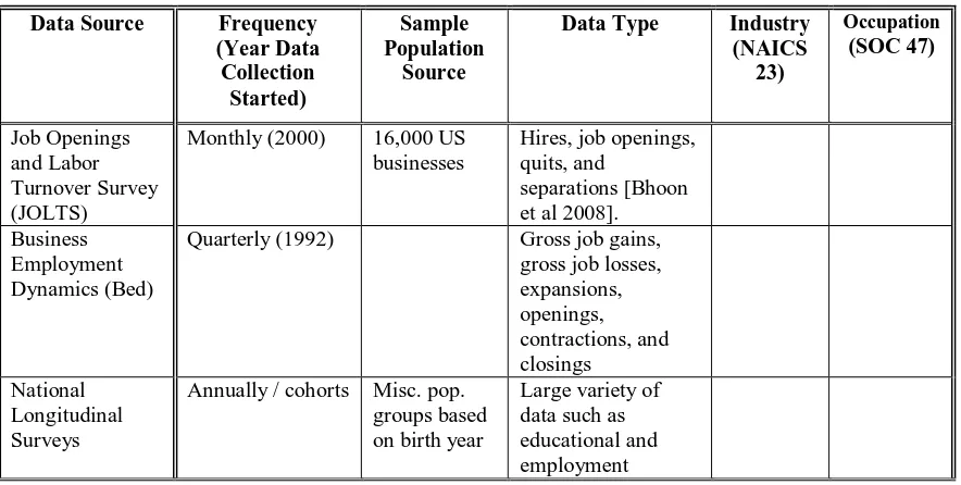
Skilled labor demand is herein considered to be the number of skilled craft workers needed to work on active construction projects. The identified sources for labor demand data are summarized in Table 2.1. The table indicates the name of the data source, the frequency at which the data are collected, the year the data collection began for the source (in parentheses), the source of the sample population, and the type of data collected.
An “X” in either the “industry” or “occupation” column indicates the data source was able to be sorted specifically by NAICS Sector 23 or SOC Division 47 respectively. For example, a data source may be able to indicate that one carpenter was employed in both a skilled labor occupation (SOC 47) and the construction industry (NAICS 23). There are skilled carpenters (SOC 47) employed in other industries, and there are other occupations employed in the construction industry (NAICS 23). Being able to select both occupation and industry separately allowed the authors to differentiate between these combinations.
The Current Population Survey (CPS) is conducted in conjunction with the USCB while all other data in the table are collected by the BLS.
Table 2.1. Evaluation of Data Sources for Labor Demand
Data Source Frequency
(Year Data Collection
Started)
Sample Population
Source
Data Type Industry
(NAICS 23)
Occupation (SOC 47)
Job Openings and Labor Turnover Survey (JOLTS)
Monthly (2000) 16,000 US
businesses
Hires, job openings, quits, and
separations [Bhoon et al 2008]. Business
Employment Dynamics (Bed)
Quarterly (1992) Gross job gains,
gross job losses, expansions, openings, contractions, and closings
National Longitudinal Surveys
Annually / cohorts Misc. pop. groups based on birth year
16
Table 2.1. Continued
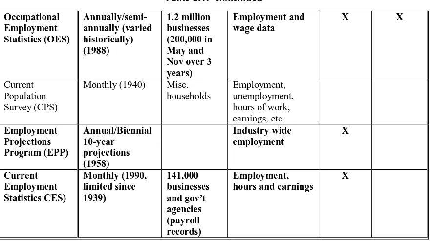
Occupational Employment Statistics (OES) Annually/semi-annually (varied historically) (1988) 1.2 million businesses (200,000 in May and Nov over 3 years)
Employment and wage data
X X
Current Population Survey (CPS)
Monthly (1940) Misc.
households
Employment, unemployment, hours of work, earnings, etc. Employment Projections Program (EPP) Annual/Biennial 10-year projections (1958) Industry wide employment X Current Employment Statistics CES) Monthly (1990, limited since 1939) 141,000 businesses and gov’t agencies (payroll records) Employment, hours and earnings
X
2.5.1.1 Occupational Employment Statistics
17
2.5.1.2 Employment Projections Program
The BLS Employment Projections Program (EPP) prepares employment outlook data about the U.S. Labor market in 10-year projections. The projections are published biennially. The projections are a function of population projections provided by the USCB and labor force participation rate projections determined by the BLS using time series adjustment techniques [Handbook 2007].
EPP data are only available annually and only for the entire construction industry. The EPP does not distinguish between skilled or non-skilled occupations and thus was excluded from further analysis.
2.5.1.3 Current Employment Statistics
The CES is a monthly survey conducted by the BLS. It “surveys about 141,000 businesses and government agencies, representing approximately 486,000 individual worksites, in order to provide detailed industry data on employment, hours, and earnings or workers on nonfarm payrolls” [BLS 2013C]. The data are based on payroll records of business establishments. Most data are available beginning in 1990, although some data has been published as far back as 1939.
The CES data can be sorted by industry (NAICS 23) but they cannot be sorted by occupation (SOC 47). Data can, however, be sorted by the designation of „production and non-supervisory employees‟ only. This category was assumed to be equivalent to skilled laborers in SOC 47. The CES is the only data source identified that has monthly data available.
2.5.1.4 Comparison Between OES and CES
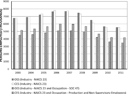
A comparison was made but the authors between the CES and OES. Data sources for both were able to be isolated by industry category, NAICS 23. During the period from 2003 to 2011, the values for number of persons employed (labor demand) at the industry level were very similar for both sources, differing by only 0 – 2% (5% in 2009).
18
analysis of the data yielded a correlation coefficient of 0.99 which indicates that the patterns in the data were similar.
Figure 2.1 shows the comparison of OES and CES data isolated by Industry (NAICS 23) only and also the comparison of OES and CES data isolated by both industry (NAICS 23) and occupation (SOC 47 or „production and nonsupervisory employees‟). Figure 2.1 shows that industry only comparison, the first set of vertical bars for each year, is almost exactly the same (0 - 2% as previously noted). Figure 2.1 also shows that the difference between both industry and occupation, the second set of vertical bars for each year, is slightly larger (10 – 20% as previously noted) but still comparable.
19
Although it would have been preferable to have data that were categorized by both NAICS 23 (industry) and SOC 47 (occupation), CES was selected as the most suitable data source for labor demand data because they were available monthly and they were comparable in magnitude to the OES which more closely met the outlined data criteria. “If, as happens frequently, a desired data series does not exist, or perhaps exists as annual data when monthly data are required, then some less perfect proxy variable must be collected instead” [Allen and Fildes 2001]. The best current source for labor demand data (the dependent variable for this research) was determined to be the Current Employment Statistics published by the BLS because the CES data represent labor demand for the desired categories (US construction industry, construction labor, skilled labor) at the desired frequency (monthly).
2.5.2 Interest Rate
Wong et al [2007] utilized the 3-month Hong Kong dollar interbank rates (HIBOR). Interbank rates are the rate at which banks buy and sell currency to each other. The most common US interest rates are Treasury notes, Federal funds rate, London Interbank offered rate (LIBOR), prime rate, and mortgage rates (variable and fixed). The LIBOR is the U.S. equivalent to the HIBOR which is published daily by the British Bankers Association (BBA) and is used as a benchmark for bank interest rates worldwide [Amadeo 2013]. The calculation of the rates involves variables such as time, maturity, and currency rates. The three-month LIBOR interest was used for this research as it was most similar to the rate used by Wong et al [2007]. But more importantly, as most other interest rates are established using the LIBOR, the LIBOR takes into account many leading trends for interest rates affecting the US economy.
20 2.5.3 Material Price
Material price data for the construction industry are available from two primary sources. The Engineering News Record (ENR) periodical publishes a Material Price Index and the BLS publishes the Producer Price Index (PPI) for industries.
ENR collects price data from 20 U.S. cities to create an index published each month. The index is based on how much it costs to purchase a hypothetical package of goods consisting of the following [ENR 2011].
0.25 short hundredweight (cwt) (0.223 long hundredweight (cwt)) of fabricated structural steel (at the 20-city average price)
1.13 tons (1,023.305 kg) of bulk Portland cement (priced locally) 1,088 board feet (2.568 cubic meters) of 2x4 lumber (priced locally)
ENR construction and building cost indexes have been issued since 1908 and 1915 respectively. The ENR indexes are used by construction industry professionals, such as cost estimators who need to account for material price escalation in project bids, researchers who create forecasts and analyze material price trends, and also government agencies such as the Bureau of Economic Analysis (BEA) which uses the ENR index to adjust construction prices.
The BLS publishes a Producer Price Index (PPI). PPI measures price change from the perspective of the seller [BLS 2013C]. The PPI is published monthly and is based on price quotation surveys of a sampling of producer firms. PPI data are published for several designations related to construction; “inputs to construction industries” was the selected designation for this research. The other construction industry related PPI designations were not considered because they dealt with new or residential construction only, maintenance and repair only, or they only began data collection in June 2010.
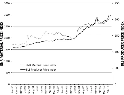
21
follow different magnitudes of scale, their patterns trend fairly similarly. The ENR index does however exhibit more variability during the 1990‟s than the BLS index. The ENR index also increase more dramatically than the BLS index around 2004 when oil prices began to increase dramatically also.
Figure 2.2. BLS Producer Price Index vs. ENR Material Price Index
Although both indexes have a long historical record, the ENR index was selected for use in the demand forecast model based on its consistency and use of the same source of prices for the research period, 1990 through 2008.
2.5.4 Construction Output
22
discussed herein. One method is to use the dollar amount expended on construction projects in a given month or year (construction spending). Another method measures the number of square feet of structure constructed (construction “size”).
Wong et al [2007] used “gross value of construction work, at constant (2000) market prices (in HK Million Dollar).” Their data sources included “all construction establishments engaged in all new architectural and civil engineering work, as well as demolition, repair, and maintenance of immobile structures.”
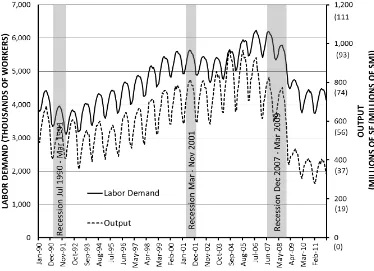
Quantifying construction output is key to understanding the demand for construction labor because they are closely correlated. The Pearson‟s Correlation Coefficient between them is 0.894 which is consistent with a strong positive association between demand and output. As the value of one variable goes up, the other variable tends to go up also. Neither variable leads nor lags the other, they rise and fall almost in unison. Figure 2.3 shows that the monthly changes in demand and output, over time, while varying in scale and magnitude, are almost identical.
23 2.5.5 Construction Spending
The USCB provides a monthly estimate of the „value of construction put in place‟ reported in dollars, similar to the value used by Wong et al (2007) for Hong Kong. “The survey covers construction work done each month on new structures or improvements to existing structures for private and public sectors” [USCB 2012A]. The „value of construction put in place‟ is a measure of the value of construction installed or erected at the site during a given period. The total value put in place for a given period is the sum of the value of work done on all projects underway during this period, regardless of when work on each individual project was started or when payment was made to the contractors. The data have been collected monthly since 1960.
In August of 1993, a new classification system was implemented by the USCB for collecting construction spending data. “The new system allows the classification of construction with one generalized coding scheme which bases project types on their end usage instead of building/non-building types” [USCB 2012B]. For example, the old classification system used the category „hospital‟ because this was the type of building. The new classification system uses the category „healthcare‟ because that is how the building will be used. The scope of this research includes data beginning in 1990, thus this change presented challenges when data published prior to 1993 were compared with data published thereafter. The USCB states that
“although some categories (lodging, office, educational, religious) seem identical to previously published data, there have been changes within the classifications that make these values incomparable. For example, private medical office buildings were classified as „office‟ buildings previously, but under the new classification these buildings are in „health care‟” [USCB 2012B].
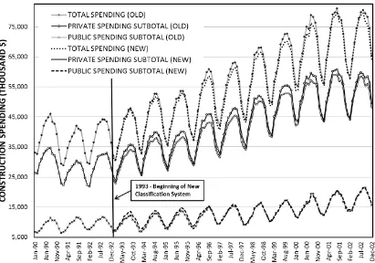
For both the old and new classification systems, an overall annual total spending value is published, and the total value is broken down into a public spending subtotal and a private spending subtotal. Each of these subtotals is broken down into residential and nonresidential categories. The non-residential category is further broken down by building types or end use, such as hospital or healthcare, as demonstrated in the following bulleted list:
TOTAL SPENDING
24 Residential Non-Residential
Educational HealthCare Etc. o PUBLIC SPENDING
Residential Non-Residential
Educational Healthcare Etc.
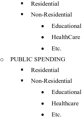
Although the classification system was changed in 1993, data were published for both the old and new classification systems through 2002. Thus we are able to compare the values of the old and new classification systems during the overlap period from 1993 through 2002. Figure 2.4 shows a comparison of the overall total spending values, and public and private spending subtotal values for the old and new classification systems from 1990 through 2002.
Figure 2.4 shows that the total spending, public spending subtotal, and private spending subtotal
values for the old and new classification systems are comparable. Although not shown in the figure, comparisons made to data broken down further than the subtotal level (i.e. building type/end use) become difficult to trace. These difficulties become further evident and are discussed in more detail in the following sections.
“The Value Put in Place Program (VIP) of the USCB has identified other problems and limitations in their data collection procedures, such as the lack of good price indexes for nonresidential construction, problems in the demarcation between structures and equipment, and the lack of a reliable annual measure in current dollars to serve as a benchmark for the monthly VIP Estimates (U.S. Census 2000)” [Rojas and Aramvareekul 2003].
25
every construction project is so diverse that data collection challenges are expected, although they are not insurmountable.
Figure 2.4. USCB Construction Spending - Old and New Classification System Comparison
2.5.5.1 Square Footage
The amount of construction built as measured by its size (expressed in square feet), is another potential type of data that could be used to quantify construction output. Possible sources of square footage construction data were investigated. Some local municipal sources were identified, as well as some association data collection efforts, but none were deemed suitable for use in this research.
26
Building Construction Cost Data annual [RS Means]. The USCB publishes the previously discussed construction spending data broken down to the building use/end type level. Combining data from these two sources could yield annual square footage of construction in the US.
The USCB publishes construction spending data and RS Means publishes median cost per square foot base size data. Matches between the two data sources were made based on the definitions provided in the USCB classification of construction document [USCB 2012C]. For example, the USCB category for office was matched up with the following RS Means building types: banks, offices - low rise, offices - midrise, and offices - high rise as shown in Table 2.2.
Table 2.2 presents some sample derivations of square footage of construction for January 2010. This month was randomly selected solely for the purpose of demonstrating the calculation. The first column presents construction put in place (spending) in dollars as published by the USCB. The second column shows the median cost per square foot as published by RS Means. The third column represents the derived square footage of construction for each USCB building type/end use category; these figures were obtained by dividing the construction put in place ($) by the square foot costs ($/SF). For construction put in place categories that were associated with more than one RS means square foot cost, the average square foot costs was used to complete the calculation. For example, five different RS Means categories – hospital, medical clinic, medical offices, living – assisted, and
nursing homes, were matched with the USCB category healthcare. The average square foot price for all four ($143.25/SF) was used to complete the derivation.
Using a non-monetary, size based metric for construction output (square footage) was determined to be better than a monetary metric in a labor demand forecasting model because three of the five model variables are already monetary (real wage, material price, and interest rate). A non-monetary measure for this variable reduces the number of monetary based independent variables thus reducing similarity and dependency.
27
derivation because there was not an applicable RS Means square foot cost, or comparable unit cost measurement (linear feet, etc.) that could be associated with them.
Table 2.2. Sample Derivation of Monthly Square Footage of Construction Using USCB and RS Means Data for January 2010
USCB Construction Put in Place – January 2010 (Millions of Dollars)
RS Means Median Cost per Square Foot 2010
($/SF ($/SM))
Derived Square Footage of Construction
(SF (SM))
Lodging 1,172 Motels 100.00 (1,076.00) 11,720,000 (1,089,000)
Office Offices, Low Rise 119.00 (1,281.00)
14,297,000 (1,328,000)
Offices, Mid Rise 117.00 (1,259.00)
Office, High Rise 150.00 (1,615.00)
Banks 187.00 (2,013.00)
2,048 Average 143.25 (1,542.00)
Health Care Hospitals 225.00 (2,422.00)
15,045,000 (1,398,000)
Medical Clinics 144.00 (1,550.00)
Medical Offices 136.00 (1,464.00)
Living - Assisted 135.00 (1,453.00)
Nursing Homes 140.00 (1,507.00)
2,347 Average 156.00 (1,679)
Thus, the data for these categories were consistently excluded from the construction output square footage data for all years. The potential model impact of each of the categories is minimal, the total for all of these categories ranged from 9 – 12 % of total construction spending in any given year. These values spiked to 14 and 15% in 2009 and 2010 respectively as there were increases in spending on highway and street, most likely as a result of the 2009 American Recovery and Reinvestment Act, more commonly referred to as the stimulus.
2.5.5.2 Comparison of Derived Square Footage Data
28
In an attempt to identify some of the specific inconsistencies, the derived square footage data were compared with the USCB construction spending data at the public and private spending subcategory level. Figure 2.5 shows construction output, at both the public and private subcategory level, expressed as: derived square feet (SF) (square meters (SM)); construction spending using the
new classification system; and construction spending using the old classification system. Figure 2.5 presents square footage calculations were completed for the entire data set, 1990 – 2011, values for the new classification system which began in 1993, and data for the old classification system which continued through 2002.
The square footage derivations trend well with the spending data with the exception of the derived values for square footage of public construction. From 1990 – 1993, the derived values are significantly higher than the public spending subcategory using the old classification system.
29
A further analysis of this inconsistency was made. Table 2.3 shows a breakdown of construction output for a sample of building type/end use categories that fall under public construction. The first two columns give the building type/end use category (e.g. buildings, hospital) and associated construction output value in January 1990 (old classification system). The third and fourth columns give the most similar corresponding building type/end use category and associated construction output value in January 1993 (new classification system).
For example, in 1990, the old classification system category title was hospital and the construction output was $227 million. In 1993, the new classification system category title is now healthcare and the construction output was $222 million. These two values are close in magnitude, but not all of the comparisons were close. The largest discrepancies between the old and new classifications systems were observed in the categories shown in bold in Table 2.3. For example, buildings and other in January 1990 total in excess of 4 billion dollars compared with office in January 1993 that totals only about 435 million dollars An attempt was made to reallocate comparable categories such that changes in the totals among categories were more similar, but the reallocation was not achievable.
Table 2.3. Comparison of USCB Public Construction Category Changes, January 1990 vs. January 1993
USCB Category Construction Output
(Millions of Dollars)
Construction Output
(Millions of Dollars)
USCB Category
January 1990 January 1993
HOUSING AND
REDEVELOPMENT
242 294 RESIDENTIAL
-- -- 6,946 NONRESIDENTIAL
Buildings 3,014 435 Office
Other 1,329
Misc. Non-building 629 148 Commercial
Industrial 118
Hospital 227 222 Healthcare
Educational 1098 1,516 Educational
Other Public 1,631 440 Public Safety
-- -- 334 Amusement & Rec
30
This assessment further confirms the USCB‟s cautionary conclusion, as previously quoted, that “although some categories (lodging, office, educational, religious) seem identical to previously published data, there have been changes within the classifications that make these values incomparable” [USCB 2012B]. This might argue for eliminating 1990 through 1992 from the data set, but we did not do so because we did not want to decrease the number of observations in the data set available for use in the forecast model.
2.5.6 Productivity
Productivity can be defined and measured in many ways. It is generally represented as some ratio or output and input. At the construction industry level, for example, productivity may be represented by construction output produced divided by the amount of labor effort required to produce that output. Allmon et al stated that some common measures of productivity are unit of labor cost (dollars per brick) or unit of output (hours per brick) [2000]. Productivity is related to labor demand in that if fewer workers are able to produce a desired output, then fewer workers will be demanded. Alternately, if the same few workers are not able to produce a desired output, then more workers will be demanded.
“Perceptions of productivity trends vary widely within engineering academia, industry, and economic academia” [Allmon et al 2000]. A paper presented by the American Association of Cost Estimators (AACE) defines productivity as “the average direct labor hours to install a unit of material” (e.g. hours / square foot) [Whiteside 2006]. The author notes that inconsistencies in measuring productivity lie in inconsistent definitions, data collection methods, utilization of common terms, and other causes. “It seems much of the problem in explaining trends in productivity is the lack of adequate productivity measures” [Allmon et al 2000]. In their study of construction labor productivity trends, Wong et al (2007) calculated an industry level measurement of productivity as construction output (Q) (in Hong Kong dollars) divided by total employed persons (L) times the median hours of work (H) represented by the following equation:
Labor Productivity = Q
L ∗ H (2.1)
31
model. Also, it seems that employed persons (L) is highly correlated with our dependent variable, labor demand. To be a good predictor in a forecasting model, productivity should be independent of other trends captured in the model by other variables.
Other researchers looked at deriving productivity data using construction industry publications such as RS Means [Goodrum, Zhai and Yasin 2009]. These efforts looked promising but were limited in scope. The research team attempted to derive a productivity measure of its own with a larger scope. The methodology and results of that analysis are currently underway and the findings will be presented in a separate paper. A paper published in 2012 quantified the impact of change on productivity which was defined as “the craft hours necessary to produce a unit of finished product” or “some relative comparison between work output and work input” [Ibbs 2012].
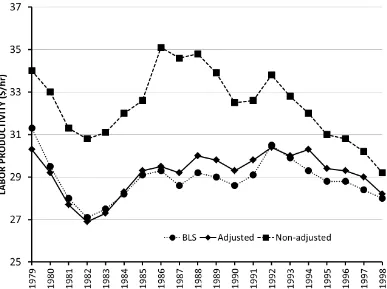
“The BLS regularly publishes productivity data for several industrial sectors. Construction is not included in this selected group of industries as the BEA considers construction data to be too unreliable to be useful in the generation of productivity data” [Rojas and Aramvareekul 2003]. This is understandable, as the construction industry is composed of many different projects varying in type, size, and cost. The collection of data over time as it relates to construction labor productivity may need to change from year to year. In manufacturing, by comparison, productivity data could be collected from the same factory from year to year. In construction the constantly changing sites and construction methods and types make this more difficult.
The BLS Division of Major Sector Productivity does, however, compile labor and multifactor productivity (MFP) measures for the construction sector (NAICS 23) as a whole. “Multifactor Productivity (MFP) relate[s] output to two or more inputs, depending on the particular multifactor productivity measure. This is in contrast to labor productivity measures, which relate output to a single input, labor” [BLS 2013D].
32 2.5.7 Real Wage
Wong et al [2007] used “median monthly employment earnings in the construction industry in [Hong King Dollars as] obtained from the General Household Survey to represent wage level.” There were several similar potential BLS sources from which real wage data for the construction industry could have been obtained for this research:
Occupational Employment Statistics (OES) Current Employment Statistics (CES)
o National Employment, Hours, and Earnings o Real Earnings Data
National Compensation Survey o Employment Cost Index (ECI)
OES data are only availably annually through 2003, and semi-annually thereafter. Also, OES data are classified using the NAICS beginning in 2002; prior to that, they were classified using the Standard Industrial Classification (SIC), the precursor to the NAICS. No OES data are available for 1996 because it was a transitional year for the survey and data prior to 1995 are limited.
BLS Real Earnings data are only available dating back to 1994 and ECI data are mostly used for setting pay levels. Therefore, the Current Employment Statistics National Employment, Hours, and Earnings were selected as the data source for real wage data. This data is available on a monthly basis and is able to be isolated at both the industry and occupation levels. Also, because CES was already selected as the data source for labor demand data, using the CES as a source for real wage data would ensure the data, at least for real wage and demand, were being compared for the same population of skilled workers.
2.6 Conclusions
33
collected, changes in category groupings and titles, and missing data years are a few examples of these challenges. Even the BLS reports challenges for those who use data such as the Occupational Employment Statistics. The value of this paper lies in its attempt to fill a significant void in documenting sources of quality construction industry data.
The data collection efforts reported here yielded quality, useable, sources and data for all six key model variables (labor demand, interest rate, material price, construction output, productivity, and real wage). Data for interest rate were straightforward to define and collect. Data for all of the other variables had one or more data sources that had to be vetted. Material price data was collected from the ENR Material Price Index. Construction output data were derived using value of construction put in place data from the USCB and RS Means cost per square foot data. Productivity was the most difficult variable to quantify as there was no widely accepted data source available. Currently, the BLS Multifactor Productivity is being used for productivity data but a derived productivity index is concurrently being studied for use in the model. The BLS Current Employment Statistics were selected as the data source for both labor demand data and real wage data.
It is important to note that where applicable, data was able to be collected specifically for SOC 47, or a similar designation. None of the data represents only the 17 specific occupations identified as skilled labor. The only data available at that level of detail was real wage.
One of the most significant results of the data collection efforts for this research project is the continuing acknowledgement that those who collect data about the construction industry need to do a better job collecting all kinds of industry data, specifically in regards to skilled labor force issues. Specifically, one or more groups need to establish specific data collection protocols and methodologies. A person or team should be tasked with collecting, managing, cataloguing, and publishing the data on a consistent basis.