Methods to Improve Prediction Accuracy under Structural Constraints.

(1)

ABSTRACT

POST, JUSTIN BLAISE. Methods to Improve Prediction Accuracy under Structural Constraints. (Under the direction of Howard Bondell.)

Statisticians are often faced with the difficult task of model selection and making inference from the selected model. A method such as Ordinary Least Squares (OLS) can be used to fit a given model but that model can often be improved by either removing some extraneous variables, shrinking parameter estimates, or by using estimates that are averages across many different models. This thesis investigates and provides new solu-tions for two common problems.

(2)

(Tib-shirani, 1996). Simulation results are given that show the usefulness of these estimators compared to their single model counterparts.

(3)

(4)

Methods to Improve Prediction Accuracy under Structural Constraints

by

Justin Blaise Post

A dissertation submitted to the Graduate Faculty of North Carolina State University

in partial fulfillment of the requirements for the Degree of

Doctor of Philosophy

Statistics

Raleigh, North Carolina 2012

APPROVED BY:

Jason Osborne Brian Reich

Yichao Wu Howard Bondell

(5)

DEDICATION

(6)

BIOGRAPHY

(7)

ACKNOWLEDGEMENTS

(8)

LIST OF TABLES

Table 3.1 Average model error and standard errors over 500 independent data sets, sample size n = 20, for the Mallows model averaged ridge re-gression estimates (MA) and the corresponding minimumCL model estimate (Best). Estimates found are model averaged over 100 equally spaced points over the degrees of freedom. Letters indicate groups of significantly different estimates. . . 45 Table 3.2 Average model error and standard errors over 500 independent data

sets, sample size n = 50, for the Mallows model averaged ridge re-gression estimates (MA) and the corresponding minimumCL model estimate (Best). Estimates found are model averaged over 100 equally spaced points over the degrees of freedom. Letters indicate groups of significantly different estimates. . . 46 Table 3.3 Average prediction error and standard error for 300 splits of the

Pakistani economic data. The training sets had 18 observations and the test sets had 10 observations. . . 47 Table 3.4 Average prediction error and standard error for 300 splits of the

Longley economic data. The training sets had 13 observations and the test sets had three observations. . . 49 Table 3.5 Average prediction error and standard error for 300 splits of the

Boston housing data. The training sets had 350 observations and the test sets had 156 observations. . . 50 Table 4.1 Average model error and standard errors over 200 independent data

sets, sample sizen = 20, coefficient vectorβ₁, for the model averaged RR estimates using AIC weights. Estimates found are the minimum AIC estimate and the model averaged estimate using a grid of 160 equally spaced points over the degrees of freedom. . . 74 Table 4.2 Average model error and standard errors over 200 independent data

sets, sample sizen = 20, coefficient vectorβ₁, for the model averaged RR estimates using AICc weights. Estimates found are the minimum AICc estimate and the model averaged estimate using a grid of 160 equally spaced points over the degrees of freedom. . . 75 Table 4.3 Average model error and standard errors over 200 independent data

(12)

Table 4.4 Average model error and standard errors over 200 independent data sets, sample sizen = 20, coefficient vectorβ₂, for the model averaged RR estimates using AIC weights. Estimates found are the minimum AIC estimate and the model averaged estimate using a grid of 160 equally spaced points over the degrees of freedom. . . 77 Table 4.5 Average model error and standard errors over 200 independent data

sets, sample sizen = 20, coefficient vectorβ₂, for the model averaged RR estimates using AICc weights. Estimates found are the minimum AICc estimate and the model averaged estimate using a grid of 160 equally spaced points over the degrees of freedom. . . 78 Table 4.6 Average model error and standard errors over 200 independent data

sets, sample sizen = 20, coefficient vectorβ₂, for the model averaged RR estimates using BIC weights. Estimates found are the minimum BIC estimate and the model averaged estimate using a grid of 160 equally spaced points over the degrees of freedom. . . 79 Table 5.1 Average model error and standard errors over 200 independent data

sets, sample size n = 20, for the model averaged LASSO estimates using Mallows criterion. Estimates found are model averaged over the ‘Break’ points, a grid of 101 equally spaced points over the ‘Frac-tion’ of the LASSO solution to the OLS solution, and the corre-sponding single ‘Best’ model estimate. Letters indicate groups of significantly different estimates. . . 91 Table 5.2 Percent of the time the model averaged LASSO estimates using

Mallows criterion and the Mallows best chosen model selected the exact true model, the percent of time these procedures included the true model, and the average number of zero estimates for coefficient vectorβ₁. . . 92 Table 5.3 Percent of the time the model averaged LASSO estimates using

Mallows criterion and the Mallows best chosen model selected the exact true model, the percent of time these procedures included the true model, and the average number of zero estimates for coefficient vectorβ₂. . . 93 Table 5.4 Percent of the time the model averaged LASSO estimates using

(13)

Table 5.5 Average model error and standard errors over 200 independent data sets, sample size n = 20, for the model averaged LASSO estimates using AIC weights. Estimates found are model averaged over the ‘Break’ points, a grid of 101 equally spaced points over the ‘Fraction’ of the LASSO solution to the OLS solution, and the corresponding single ‘Best’ model estimate. Letters indicate groups of significantly

different estimates. . . 95

Table 5.6 Average model error and standard errors over 200 independent data sets, sample size n = 20, for the model averaged LASSO estimates using AICc weights. Estimates found are model averaged over the ‘Break’ points, a grid of 101 equally spaced points over the ‘Fraction’ of the LASSO solution to the OLS solution, and the corresponding single ‘Best’ model estimate. Letters indicate groups of significantly different estimates. . . 96

Table 5.7 Average model error and standard errors over 200 independent data sets, sample size n = 20, for the model averaged LASSO estimates using BIC weights. Estimates found are model averaged over the ‘Break’ points, a grid of 101 equally spaced points over the ‘Fraction’ of the LASSO solution to the OLS solution, and the corresponding single ‘Best’ model estimate. Letters indicate groups of significantly different estimates. . . 97

Table 6.1 Table of Cell Means forθ1 . . . 125

Table 6.2 Table of Cell Means forθ2 . . . 126

Table 6.3 Null Model Simulation Results . . . 127

Table 6.4 Simulation Results for Effect Vectorθ1. There are 23 truly nonzero level differences and 11 level differences that should be collapsed. There are 68 truly nonzero pairwise differences and 71 pairwise differences that should be collapsed. . . 128

Table 6.5 Simulation Results forθ2. There are 18 truly nonzero level differences and 16 level differences that should be collapsed. There are 61 truly nonzero pairwise differences and 78 pairwise differences that should be collapsed. 129 Table 6.6 Table of Cell Means forθ3 . . . 130

Table 6.7 Simulation Results forθ3 with error variance one. There are three truly nonzero level differences and three level differences that should be col-lapsed. There are three truly nonzero pairwise differences and 11 pairwise differences that should be collapsed.. . . 131

(14)

(15)

LIST OF FIGURES

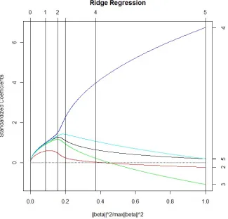
Figure 3.1 Ridge regression solution path for the full Pakistani economic data. Tick marks along the top of the graph represent where the ridge regression estimate has a given number of effective degrees of free-dom. Tick marks along the right of the graph represent the full least squares solution with the following: 1=Land Cultivated, 2=Infla-tion Rate, 3=Number of Establishments, 4=Popula2=Infla-tion, and 5=Lit-eracy Rate. . . 47 Figure 3.2 Ridge regression solution path for the full Longley economic data.

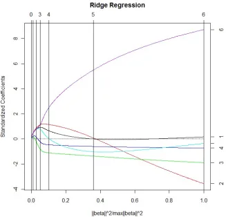
Tick marks along the top of the graph represent where the ridge regression estimate has a given number of effective degrees of free-dom. Tick marks along the right of the graph represent the full least squares solution with the following: 1=Gross National Prod-uct implicit price deflater, 2=Gross National ProdProd-uct, 3=number of unemployed, 4=number of people in the armed forces, 5=‘non-institutionalized’ population at least 14 years of age, and 6=year. 48 Figure 4.1 Ridge regression profile forβ₁ from the simulation done in section

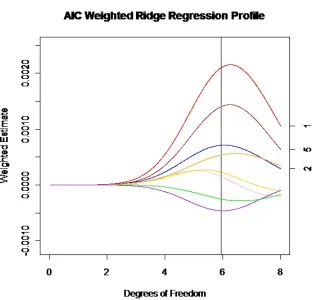
4.6. The number on the right of the graph describes which regres-sion parameter (1-8) path the curve represents. The three vertical lines give the minimum AIC, AICc, and BIC chosen estimates. . . 68 Figure 4.2 AIC weighted ridge regression profile for β₁ from the simulation

done in section 4.6. The model averaged ridge regression estimate is given by the area under the curves. . . 69 Figure 4.3 AICc weighted ridge regression profile for β₁ from the simulation

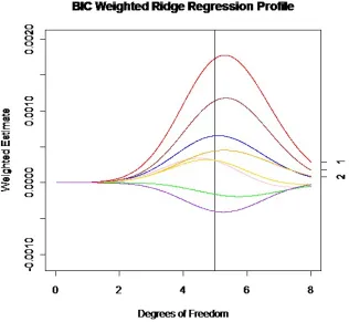
done in section 4.6. The model averaged ridge regression estimate is given by the area under the curves. . . 70 Figure 4.4 BIC weighted ridge regression profile for β₁ from the simulation

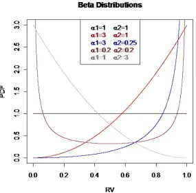
done in section 4.6. The model averaged ridge regression estimate is given by the area under the curves. . . 71 Figure 4.5 Plots ofBetadistributions for different values of the shape

param-eters α1 and α2. . . 72

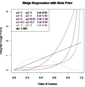
Figure 4.6 Weighted ridge regression profiles for a one predictor example along with their Betaweighted estimates . . . 73 Figure 5.1 LASSO solution path for Pakistani economic data. Tick marks

(16)

Chapter 1 Introduction

Statisticians are often faced with the difficult task of model selection and making inference from the selected model. The topic of model selection has received much atten-tion in the statistical literature. Historically hypothesis testing methods were the focus, however in recent decades there have been many developments on the topic that uti-lize regularization, or penalization, methods. Given a response and predictor variables, a method such as ordinary least squares (OLS) can be used to fit a given model. The fit of this model can often be improved upon by removing some extraneous variables, using estimates that are averages of estimates across different models, or shrinking the esti-mates in some way. This thesis investigates and provides new solutions for two common problems in this area.

1.1 Regularization Framework

(17)

1, ..., n,a general one dimensional regularization problem has the form

min f∈H

" _n X

i=1

L(yi, f(Xi)) +λJ(f)

#

,

where L(·,·) is a loss function, f(·) is a function in some space of functions H, λ is a tuning parameter, and J(f) is a penalty functional (Hastie et al., 2009).

Many common methods used today fall into this framework including ridge regression (RR) (Hoerl and Kennard, 1970), the least absolute shrinkage and selection operator (LASSO) (Tibshirani, 1996), least angle regression (LARS) (Efron et al., 2002), and the elastic net (EN) (Zou and Hastie, 2005) (involves a two-dimensional functional with two tuning parameters) to name a few.

1.2 Plan of Dissertation

This thesis lays out new solutions that utilize the regularization framework for two common problems statisticians face. The first problem is that of improving the prediction accuracy of our model estimates. We develop a method that combines ridge regression and frequentist model averaging (FMA). The second problem is that of choosing the important factors in multi-factor analysis of variance (ANOVA) and deciding which levels of the factors are significantly different from one another when interactions are included in the model. We develop a new penalization method that simultaneously selects important predictors and also creates non-overlapping groups of levels within each factor.

(18)

Chapter 5 discusses the extensions of FMA to the LASSO procedure. In chapter 6, the grouping and selection using heredity (GASH) ANOVA method is introduced as a solution to the multi-factor ANVOA with interaction problem.

(19)

Chapter 2 Introduction to Model Averaging

Consider the regression setup with n independent observations, each consisting of a response variable yi and a countably infinite number of predictors Xi = (xi1, xi2, ...)T,

i= 1, ..., n. Assume the true model for the data can be written as

yi =µi+i = ∞

X

j=1

βjxij +i

and in vector form as

y=µ+,

where y = (y1, ..., yn)T, µ = (µ1, ..., µn)T, β1, β2... are regression parameters, and =

(1, ..., n)T are error terms. In practice, we often approximate µusing a finite number of predictors pn, which we can write in matrix form as

(20)

whereµi is approximated byPp_jn₌₁βjxij,X is a n×pn design matrix with (i, j) element xij, and β= (β1, ..., βpn)

T_.

The standard way to fit the linear model above is using ordinary least squares (OLS). The OLS model fitting criterion is given by

min

β ||y−Xβ||

2

and, when X is full rank, the OLS solution is given by βb_OLS = (XTX)−1XTy. The

OLS solution can often be improved upon in terms of prediction accuracy and inter-pretation (Burnham and Anderson, 2002). Interinter-pretation of the estimates can be aided by eliminating some of the predictors from the model. Prediction accuracy can be im-proved by trading increased bias for lower variance. The OLS estimates are unbiased, but when many correlated predictors are included in the model the estimates may have high variance. There are many methods for selecting the structure and fit of the model. For example, on can use best subset selection, forward/backward stepwise selection, or any of the regularization methods mentioned in chapter 1.

These methods all have some criteria such as hypothesis tests or a tuning parameters that control the final model and model fit selected. Once a procedure is applied and the model and fit are selected, inference usually proceeds conditional on this result. Thus, this aspect is often treated as known in advance. This can lead to invalid inference because the variability inherent in the model selection process is ignored, i.e. if another data set was available and the selection procedure applied to that data set, a different structure or fit would likely be chosen.

(21)

formulas, another is to use bootstrapping to assess the variability, and the third is to use model averaging. Model averaging usually does not help in terms of interpretability of the model, but, if the goal is to predict for new responses, model averaging tends to yield very good prediction accuracy. Note that while this is being called ‘unconditional infer-ence,’ the inference is of course conditional on the overall set of models being considered. Model averaging is most often done in a Bayesian framework and is called Bayesian model averaging (BMA). However, there is an increasing amount of literature in the last decade on frequentist model averaging (FMA) (Wang et al., 2009). We now give a brief review of BMA (for in depth reviews of theory and application see Hoeting et al. (1999) and Clyde and George (2004)) followed by a more in depth review of FMA.

2.1 Bayesian Model Averaging Review

The Bayesian paradigm gives a strong and natural theoretical approach to incorporat-ing model and parameter uncertainty into inference, yieldincorporat-ing the unconditional inference we desire. There has been extensive work done in the area of BMA, especially as of late due to the advances in computing power and Markov chain Monte Carlo (MCMC) methods (Clyde and George, 2004).

2.1.1 The BMA Framework

(22)

Mm by P(Mm) and the prior for the parameters of that model by P(βm|Mm). We denote the combination of our data as Z = (X,y). Hence, for model Mm we have the joint distribution

P(Z,β_m,Mm) = P(Z|βm,Mm)P(βm|Mm)P(Mm),

where P(Z|β_m,Mm) is the distribution or likelihood of the data. Following Clyde and George (2004), this places all of the models into a hierarchical mixture model framework where the data come from first generating the model Mm from the candidate model set, then generating the parameter vectorβ_m for that model, and finally generating the data fromP(Z|β_m,Mm).

Using Bayes rule the posterior probability for model Mm is given by P(Mm|Z) =

P(Z|Mm)P(Mm)

PM

k=1P(Z|Mk)P(Mk) ,

where P(Z|Mm) =

R

P(Z|β_m,Mm)P(βm|Mm)dβm (throughout we assume a continu-ous distribution but the definition for a discrete distribution is straightforward). These posterior model probabilities can be used to select a single best model, compare models, or combine models using model averaging. If one model has a much higher posterior prob-ability or if a few models have high posterior probprob-ability these models can be selected and reported. To compare model j to model m, a Bayesian would usually look at the posterior odds of the two models defined as

P(Mj|Z) P(Mm|Z)

= P(Z|Mj)P(Mj) P(Z|Mm)P(Mm)

(23)

When the prior probabilities of the two models are the same they cancel and we are left with what is known as the Bayes factor. The Bayes factor describes the level of support for one model over another utilizing just the data at hand. The Bayes factor can sometimes be difficult to find exactly. For large sample sizes Schwarz (or Bayes) information criterion (BIC), given by BIC = −2log(L) +log(n)pn (Schwarz, 1978) where L is the likelihood of the data, offers a good approximation to the posterior probability for a given model:

P(Mm|Z)≈

exp(−BICm/2)P(Mm)

PM

k=1exp(−BICk/2)P(Mk)

,

where BICm denotes the BIC value for model m. For this reason, the ratio of the expo-nentiated BIC values is often used to approximate the Bayes factor (Kass and Raftery, 1995).

To make inference for a particular quantity of interest η, one would look at the pos-terior distribution ofη (Hoeting et al., 1999). This is given by

P(η|Z) = M

X

m=1

P(η|Mm,Z)P(Mm|Z).

This posterior distribution is an average of the posterior distributions under the different models weighted by their posterior model probabilities. The mean and variance of this posterior distribution are given by

E[η|Z] = M

X

m=1

(24)

and

V ar[η|Z] = M

X

m=1

V ar[η|Z,Mm] +E[η|Z,Mm]

2

P(Mm|Z)−E[η|Z]

2

.

It has been shown that by using these averaged estimates one tends to see better perfor-mance in terms of predictive ability than using an estimate from a single model (Madigan and Raftery, 1994).

The main issues and drawbacks associated with BMA are the posterior calculations and the prior model specifications (Clyde and George, 2004). The posterior calculations require evaluating integrals for each model in the candidate set that rarely have closed forms. This limitation has been somewhat eased by the recent advances in computational speed and in MCMC methods. However, MCMC methods have their own difficulties such as identifiability issues and determining if the distributions have converged (Eberly and Carlin, 2000). The other main issue is the difficulty that comes is specifying meaningful and non-conflicting prior distributions for the models and their parameters. This becomes more difficult when M is very large.

2.2 Frequentist Model Averaging Review

(25)

estimators using a local misspecification framework. Because our focus is on the linear regression model, we choose to define the FMA estimators in this framework.

The basic reason for using FMA is to provide more robust results. Recall we suppose that there are M candidate models under consideration. When only considering linear mean structures, theM models usually arise from including or excluding predictors from the models (including derived predictors such as interactions or quadratic terms). Again, letβj represent the effect for the same predictor in each of theM models. We define the FMA estimate for βj, j = 1, ..., pn as

ˆ ¯ βj =

M

X

m=1

wmβˆj,m,

where wm is a weight for model m,

PM

m=1wm = 1, and ˆβj,m is the estimate for βj under the mth model (if the corresponding predictor is not in model m, ˆβj,m is set to zero).

Another technique for performing FMA is to average the predicted responses rather than the regression coefficients. In the context of the linear model, these two methods are equivalent. Also, we make note that by setting the weight for a single model to one, the usual approach of selecting one ‘best’ model falls into the FMA framework.

(26)

2.2.1 Information Theory Weights

The first type of fixed weight we review was developed by Buckland et al. (1997), which are based around information theory. Information theory gives a strong theoretical basis for model selection so we briefly describe the approach before giving the weights.

Information theorists do not believe that a ‘true’ model exists, rather they believe in an abstract notion of truth (call this f) that is being approximated by a model g (Burnham and Anderson, 2002). The Kullback-Leibler (KL) distance betweenf and g is defined generally for continuous functions as

I(f, g) =

Z

f(Z)log

f(Z) g(Z|θ)

dZ,

whereZis the data andθis the parameter vector for the approximating modelg. The KL distanceI(f, g) denotes the information lost wheng is used to approximate f. Given the data Z with sample size n and the class of models g(Z|θ), there exists a conceptual KL best model g(Z|θ0). The connection between KL distance and the maximum likelihood

estimate (MLE) ofθ, ˆθM L, is that ˆθM L converges toθ0 asymptotically and bias of ˆθM Lis with respect to θ0. This connection between likelihood inference and information theory

creates a basis for using information theory for model selection.

Due to the fact that f is unknown, we cannot estimate I(f, g). However, by noting that

I(f, g) = Ef[log(f(Z))]−Ef[log(g(Z|θ))] =C−Ef[log(g(Z|θ))],

where C is a constant, one can estimate a relative distance to compare models. This quantity is minimized at θ0, but we must estimate θ by some ˆθ. Therefore, to use KL

(27)

estimated expected KL distance. Therefore, the critical issue is to estimate

EZ∗ h

EZ h

loggZ|θˆ(Z∗)ii,

where Z and Z∗ are independent random samples and the expectations are both with respect to f (Akaike, 1973).

By use of Taylor expansions and other approximations (Burnham and Anderson, 2002), it can be shown that an unbiased estimator of our target is

loggZ|θˆ(Z)−trˆ J(θ0) [I(θ0)]

−1

,

where tr stands for the trace,

J(θ0) =Ef

(

∂

∂θlog(g(Z|θ))

∂

∂θlog(g(Z|θ)) T)

θ=θ0 ,

and

I(θ0) = Ef

−∂

2_log_(g(_Z_|_θ₎₎

∂θi∂θj

θ=θ0 .

Iff is in the set of modelsg, then J(θ0) =I(θ0) and the trace term is simply the length

of the parameter vector, pn. Although this is not likely to be the case, the use of pn as an estimate of the trace term is still a good estimate (Shibata, 1989). Note thatθ should include the error varianceσ2 if it is unknown (makingpnfrom abovepn+ 1). By using pn as the estimate and multiplying by negative two we get the usual Akaike’s information criterion (AIC) (Akaike, 1974),

(28)

Thus, the use of AIC for model selection has strong theoretical underpinnings.

For their weights, Buckland et al. (1997) decided to use the class of information criteria of the form

IC =−2log(L) +Q(n, pn),

where L represents the likelihood for the model and Q(n, pn) is a penalty function that can depend on the sample size n and the number of parameters pn. To compare model j to model m using this criterion, one can look at the ratio,

Ljexp(−Qj/2) Lmexp(−Qm/2)

= exp(−ICj/2) exp(−ICm/2)

,

where Lm, Qm, and ICm are the likelihood, penalty function, and IC for model m re-spectively. This led to the model averaging weight for model m given by

wm =

exp(−ICm/2)

PM

k=1exp(−ICk/2)

.

Burnham and Anderson (2002) modified these weights using the ‘AIC differences,’ ∆AIC_m = AICm −AICmin, where AICm is the AIC for model m and AICmin is the minimum of the AIC estimates over the model set M. They advocate using these AIC differences to rank the different candidate models and to form equivalent (when Q cor-responds to AIC) but more easily interpreted weights which they call ‘Akaike weights’ given by

wm =

exp −∆AIC_m /2

PM

k=1exp(−∆AICk /2) .

(29)

the candidate model set. If desired, the weights can be redefined with prior probabilities, P(wm), for the models. The weights are then given by

wm =

exp(−∆m/2)P(wm)

PM

k=1exp(−∆k/2)P(wk) .

Note that these weights do not fully satisfy the BMA scheme because prior distributions on the parameters are also needed (Burnham and Anderson, 2002).

Differences of this form can be found and used for any choice of penalty Qin the IC class and we shall use this form of the weight. Typical penalty functions used for Q are the BIC and AIC penalties already discussed as well as the small sample correction to AIC in the linear model with homoskedastic errors called AICc (Hurvich and Tsai (1989) and Hurvich and Tsai (1995)). The AICc criterion is given by

AICc=AIC +2pn(pn+ 1) n−pn−1

.

When selecting a single best model AIC tends to perform poorly when the ratio of the sample size to the number of parameters is small (< 40). Therefore, AICc is recom-mended in this case as it has been shown to perform better than AIC for small samples even when its assumptions are not met (Burnham and Anderson (2002) and Sakamoto et al. (1986)). The same is likely true when using these values for model averaging.

(30)

AIC Weights in the BMA Framework

The AIC weights (and AICc weights) can be motivated from the Bayesian point of view (Burnham and Anderson, 2002). If the approximation to the Bayesian posterior model probability utilizing BIC is used, a savvy prior for the models yields the AIC weights. Let the prior weight for model Mm be given by

P(Mm)∝exp ∆BICm /2

exp −∆AIC_m /2,

where ∆BIC_m is the BIC difference for model m. Thus, using these priors it is easily seen that

P(Mm|Z)≈

exp −∆BIC_m /2P(Mm)

PM

k=1exp(−∆BICk /2)P(Mk)

= exp −∆ AIC m /2

PM

k=1exp(−∆AICk /2)

=wm.

This prior does not depend on the data, only the sample size and number of parameters.

2.2.2 Bootstrap Weights

(31)

are used to obtain estimates of uncertainty about some quantity of interest fromh. This set of bootstrap samples acts as a set of independent real data samples from h. The behavior of the estimator on truly independent data sets from h can then be deduced from its behavior over the bootstrap samples.

For example, suppose one wished to estimate the variance of an estimator ˆψ given a sample of size n arising from some distribution h. If the estimate is complicated, the theoretical variance may be very difficult to find analytically. Instead, one might use the nonparametric bootstrap method. First, one would create B bootstrap samples each of sizenby sampling with replacement from thenobserved values (randomly sampling from the empirical distribution of the data). The recommended number of bootstrap samples is anywhere from B = 1000 to B = 10,000. The estimator of interest would then be calculated on each bootstrap sample, call these estimators ˆψb, b = 1, ..., B. Finally, to make inference about the variance of the estimator one could look at the sample variance of the bootstrap estimators,

s2_boot =

PB

b=1( ˆψb−ψ)ˆ¯ 2 B−1 , where ˆψ¯ is the sample mean of the bootstrap estimates.

(32)

are then ranked in terms of some criterion (such as minimum AIC, AICc, BIC, Mallows CP or cross validation value) and one model selected as the ‘best’. The model selection relative frequency for model m given by

wBoot_m = frequency of selection/B

can be estimated and used as a model weight. These model selection relative frequencies were shown to give positive results that were similar to using IC weights, although not identical (Burnham and Anderson, 2002).

2.2.3 Cross Validation Weights

The first type of adaptive weight we discuss are weights based on Cross Validation (CV) and the Jackknife. CV is a method to assess the performance of a model or to select model parameters. The idea has been around in some form since the 1930’s, but k-fold CV was first clearly brought forward in the late 1960’s and 1970’s. The method of CV is relatively straight forward procedure that is one of the most widely used (Hastie et al., 2009) and we describe it here.

(33)

is used to evaluate the prediction error on that fit. The prediction errors for each fold are then averaged and this value is used as the estimate of prediction error. If there is a tuning parameter, this process is done for many different values of the tuning parameter. The tuning parameter that yields the smallest estimated prediction error is the value chosen.

There is no optimal choice for the number of foldsk. However, 5-fold or 10-fold CV is often used. The jackknife is a similar procedure that is also known as leave one out CV (LooCV), as it uses n as the number of folds.

Weights using these methods have been created. The adaptive regression by mixing (ARM) procedure (Yang, 2001) uses CV weights to combine different regression models. The ARMS procedure (Yuan and Yang, 2005) adds in a screening step that uses AIC or BIC. These procedures were shown to have a desirable risk bound. Hansen and Racine (2009) defined weights based on the jackknife criterion which they termed Jackknife Model Averaging that, under suitable conditions, were also shown to have desirable risk and loss properties.

2.2.4 Mallows Criterion Weights

Hansen (2007) proposed minimizing MallowsCP criterion to select the weight vector for combining subset regressions. Mallows (1973) described a useful statistic for assessing the fit of a model called the CP statistic (known commonly as Mallows CP). Denote a subset of the predictors by P, the number of predictors in that subset by |P|, and the least squares estimate on that subset by ˆβ_P. Mallows CP criterion is given by

CP = 1 ˆ σ2

y−X

ˆ

β_P

2

(34)

where ˆσ2 _{is an estimate of the error variance} _σ2_.

Let our model set Mbe a (possibly infinite) sequence of candidate models where the mth _{model uses any}_k

m >0 regressors. The mth candidate model is given by

yi = km

X

j=1

βj(m)xi,j(m)+vi(m)+i (2.1) and we define the approximation error vi(m) by

vi(m) =µi− km

X

j=1

βj(m)xi,j(m).

Using matrix notation, model 2.1 can be rewritten as

y=µ+=Xmβm+Vm+.

Here Xm is an n × km matrix with ijth element xi,j(m) and Vm = (v1(m), ..., vn(m))T.

Define ˆβ_m,OLS to be the OLS solution for the mth candidate model. Thus, we have an estimate for µ from themth candidate model,

ˆ

µ_m =Xmβˆm,OLS =Xm(XmTXm)−1XTmy=Pmy, where Pm is the usual ‘hat’ matrix.

The Mallows model averaged estimate of µ is defined as

ˆ

µ(w) = M

X

m=1

(35)

The choice of weight vector is then chosen adaptively using a Mallows type criterion given by

Cn(w) = (y−µˆ(w))T(y−µˆ(w)) + 2σ2tr(P(w)). The estimated weight vector is given by

ˆ

w = argmin

w

Cn(w),

the estimate of µis ˆµ( ˆw), and the estimate for β is given by

ˆ

β_{M allows} = M

X

m=1

ˆ

wmβˆm,OLS.

(36)

Chapter 3 Model Averaged Ridge Regression

3.1 Introduction and Motivation

Consider the regression setup with n independent observations, each consisting of a response variable yi and a countably infinite number of predictors Xi = (xi1, xi2, ...)T,

i= 1, ..., n. The true model for the data can be written as

yi =µi+i = ∞

X

j=1

βjxij +i

and in vector form as

y=µ+,

where y = (y1, ..., yn)T, µ= (µ1, ..., µn)T, = (1, ..., n)T, βj are the regression param-eters, E(i|Xi) = 0, and V ar(i|Xi) =σ2. In practice, we approximate µ using a finite number of predictors pn, which we can write in matrix form as

(37)

whereµi is approximated byPp_jn₌₁βjxij,X is a n×pn design matrix with (i, j) element xij, and β= (β1, ..., βpn)

T_.

The standard way to fit the linear model above is using ordinary least squares (OLS). The OLS model fitting criterion is given by

min

β ||y−Xβ||

2

and, in the full rank case, the OLS solution is given by βb_OLS = (XTX)−1XTy. The

OLS solution can often be improved upon in terms of prediction accuracy and interpre-tation (Burnham and Anderson, 2002). Interpreinterpre-tation of the estimates can be aided by eliminating some of the predictors from the model. Prediction accuracy can be improved by trading increased bias for lower variance. The OLS estimates are unbiased, but when many correlated predictors are included in the model the estimates may have high vari-ance. There are many methods for selecting the structure and fit of the model such as best subset selection, forward/backward stepwise selection, ridge regression (RR), the least absolute shrinkage and selection operator (LASSO) (Tibshirani, 1996), the elastic net (EN) (Zou and Hastie, 2005), and least angle regression (LARS) (Efron et al., 2002) to name a few. In this paper, our goal will be that of improving the prediction accuracy of our estimates.

(38)

vector. The ridge regression solution in Lagrangian form is given by

b

β_RR = min

β ||y−Xβ||

2

+λβTβ,

whereλ >0 is a tuning parameter. The closed form solution is given byβb_RR = (XTX+

λIpn)

−1_XT_y_{. A nice property of ridge regression is that} _β

RR exists even when pn> n. If the true mean is in the linear space spanned by the observed predictors, i.e.µ=Xβ, ridge regression has been shown to have favorable properties. The mean square error (MSE) of the ridge estimator is

M SE(βb_RR) = (Bias of βb_RR)2+V ar h

b β_RR

i

=λ2βT(XT_X₊_λ_I pn)

−1₍_XT_X₊_λ_I pn)

−1_β₊_σ2₍_XT_X₊_λ_I pn)

−1_XT_X₍_XT_X₊_λ_I pn)

−1_.

It is well known that the OLS solution is unbiased and has variance σ2 _XT_X−1

. We can see that compared to the OLS estimate, the ridge regression estimate increases the bias but decreases the variance by adding a term to the diagonal of the XTX matrix. This is commonly referred to as a bias-variance trade-off. In the seminal ridge regression paper by Hoerl and Kennard (1970), it was shown that there exists λ values such that

b

β_RR obtains a lower total MSE than βb_OLS. This result was extended to a more general

MSE type criterion by Theobald (1974). Lee and Triveld (1982) also showed a similar result when the errors are correlated.

(39)

numer-ical studies the author also investigated the multiple parameter case and showed that the range in which the ridge regression estimate had lower MSE than the OLS estimate was larger in the omitted variable situation than in the standard full predictor situation. Thus, ridge regression provides an interesting and useful alternative to OLS.

Although ridge regression has desirable properties, as with many penalized regression methods there exists the difficulty of selecting the tuning parameter. Many different nat-ural choices for λ have been suggested and compared (for example see Gibbons (1981), Golam Kibria (2003), and Alkhamisis and Shukur (2007)), although the more common analysis is to select the tuning parameter based upon minimizing a criterion such as Mal-lows CL, Akaike’s information criterion (AIC), Bayes information criterion (BIC), cross validation (CV), or generalized cross validation (GCV). Li (1986) showed in the context of choosing the ridge tuning parameter that both Mallows CL and GCV are asymptoti-cally optimal in terms of achieving the optimal loss. Once the tuning parameter is chosen, inference for the selected model (usually prediction) often proceeds conditional on the chosen model selection criterion, treating this aspect as known in advance. However, there is inherent variability in the selection of the tuning parameter, i.e. if another data set from the same population was available and the selection procedure was applied to that data set, a different tuning parameter would likely be chosen.

(40)

of frequentist model averaging (FMA). Section 3.3 delves into the details of the model averaged ridge regression estimator. The choice of weights that are often used for FMA are discussed in section 3.4. The use of Mallows Criterion to select the weight vector is discussed in section 3.5. Section 3.6 shows the connection between our estimate and Bayesian linear regression. We give the asymptotic theory of our estimator in section 3.7. In sections 3.8 and 3.9, the Mallows model averaged ridge regression estimate demon-strated using Monte Carlo simulation studies and real data examples. Finally, a brief discussion is given in section 3.10.

3.2 FMA Review - Basic Paradigm

Model averaging is most often done in a Bayesian framework and is called Bayesian model averaging (BMA). There is a large literature on the topic (for a good review see Hoeting et al. (1999)). BMA has the drawback that an investigator has to pick prior probabilities for the set of candidate models and for the parameters of each model. This can often lead to conflicting priors (Hjort and Claeskens, 2003). In the case of ridge re-gression this is not a difficulty since there is only one model being considered. In fact, the usual Bayesian ridge regression estimate is a model averaged estimator in the sense we are considering in this paper. We discuss the Bayesian formulation for ridge regression in section 3.6. Recently there has been an increase in papers on the topic of frequentist model averaging. Our paper follows this approach, which we give a brief review of here (see Wang et al. (2009) for a more thorough review).

(41)

regression procedures (Yang, 2001). Hjort and Claeskens (2003) give asymptotic theory for FMA estimators using a local misspecification framework. Because our focus is on the linear regression model, we choose to define the FMA estimators in this framework. The basic reason for using FMA is to provide more robust results. The traditional FMA paradigm supposes there are M candidate models being considered. When only considering linear mean structures, the M models usually arise from including or ex-cluding predictors from the models (inex-cluding derived predictors such as interactions or quadratic terms). Letβj be a regression parameter that represents the effect for the same predictor in each of the M models. We define the FMA estimate for βj, j = 1, ..., pn as

ˆ ¯ βj =

M

X

m=1

wmβˆj,m,

where wm is a weight for model m,

PM

m=1wm = 1, and ˆβj,m is the estimate for βj under the mth model (if the corresponding predictor is not in model m, ˆβj,m is set to zero).

Another technique for performing FMA is to average the predicted responses rather than the regression coefficients. In the context of the linear model, these two methods are equivalent. Notice that by setting the weight for a single model to one, the usual approach of selecting one ‘best’ model falls into the FMA framework. There are many different methods for selecting the weight vector. We delay the discussion of this topic until section 3.4.

3.3 Adapting FMA to Ridge Regression

(42)

model fits on the same model structure to choose from. These model fits are controlled by the tuning parameter λ. Thus, instead of a weighted sum across different models as our estimator for βj, we really require a weighted integral over the tuning parameter λ. Specifically, the model averaged ridge regression estimator we desire is given by

ˆ ¯ βj =

Z ∞

0

w(λ) ˆβj,RR(λ)dλ,

where

Z ∞

0

w(λ)dλ = 1

and ˆβj,RR(λ) is the ridge regression estimate of βj for a given choice of λ.

Alternatively, we can define the model averaged ridge regression estimator based on a transformation ofλthat has finite support given by [0, pn]. Letτ =

Ppn j=1

δj

δj+λ, whereδ1 ≥ δ2, ..., .δpn ≥0 are the eigenvalues of X

T_X

. We can see that when λ= 0, corresponding to the full least squares estimate, we have τ = pn. When λ = ∞, corresponding to the null solution, we have τ = 0. Thus, we can rewrite our solution as

ˆ ¯ βj =

Z pn

0

w(τ) ˆβj,RR(τ)dτ,

where

Z pn

0

w(τ)dτ = 1.

(43)

assume that the predictors have been standardized so that

XT_X ₌

   1 ρ ρ 1   ,

i.e.XT_X _{is in correlation form where}_ρ_{is the correlation between the predictors. Denote} the eigenvalue decomposition of XT_X _by _Q_∆_QT_{, where} _Q _{is the orthogonal matrix} of eigenvectors of XT_X _(since _XT_X _{is symmetric) and ∆ is the diagonal matrix of} eigenvalues of XT_X _{with eigenvalues} _δ

1 and δ2. We can easily derive the eigenvalues in

this simplified case asδ1 = 1 +ρandδ2 = 1−ρ. By rewriting Ipn asQQ T

any particular ridge regression solution can be written in the form

Q 

 

1

1+ρ+λ 0 0 ₁₋1_ρ₊_λ



 Q

T_XT_y_. _(3.1)

Meanwhile, a model averaged ridge regression estimator is of the form

Q    R∞ 0

w(λ)

1+ρ+λdλ 0 0 R₀∞₁₋w(_ρλ₊)_λdλ



 Q

T_XT_y_. _(3.2)

By simple algebra we can rewriteR₀∞ ₁₊w_ρ(λ₊)_λdλas ₁₊_ρ1₊_κ1 andR₀∞₁w₋(_ρλ₊)_λdλas ₁₋_ρ1₊_κ2, where κ1 =

"

1

R∞

0

w(λ) 1+λ/(1+ρ)dλ

−1

#

(1 +ρ)

and

κ2 =

"

1

R∞

0

w(λ) 1+λ/(1−ρ)dλ

−1

#

(44)

Thus, our estimate does not simply yield another ridge regression solution. We only get back a particular ridge regression solution if κ1 = κ2, which only occurs if we have

orthogonal (ρ= 0) predictors or all weight is placed on a single model.

We make note that this model averaged ridge regression estimate is in the form of a generalized ridge regression estimator (Hoerl and Kennard, 1970) with tuning parameters κ1 ≥0 and κ2 ≥0. We cannot obtain any arbitrary generalized ridge regression solution

in this way due to the fact that κ1 and κ2 are related. For any ρ6= −1,1, either tuning

parameter can be zero only if full weight is put on the model with λ = 0 (implying both κ1 and κ2 would be zero). The relationship of the parameters is symmetric with

respect to ρ. For correlations close to zero the parameters tend to be close together and move further apart as the magnitude of the correlation approaches one. The form of the generalized ridge regression tuning parameters for a general problem can be written as

κj =

"

1

R∞

0

w(λ) 1+λ/δjdλ

−1

#

δj,

where δj is the jth eigenvalue of XTX. Therefore, we can see that our model averaged ridge regression estimator yields a generalized ridge regression estimator at some point along a particular path in the space of generalized ridge regression solutions.

3.4 Weight Choice

(45)

the weights is important as different methods have different properties. Most of the weighting structures used for the usual FMA estimators can be applied to model averaging a ridge regression fit. This can be done by approximating the model averaged ridge regression estimator’s integral by fitting a grid of solutions over different values of the tuning parameter and treating these solutions as the candidate models. The selection of weight vectors for FMA estimators is still an active area of research which we give a brief review of here.

3.4.1 Fixed Weights

Buckland et al. (1997) proposed calculating an information criteria for each model and using weights based on these values. The form of the weights they advocate is

wm =

exp(−ICm/2)

PM

m=1exp(−ICm/2) ,

where ICm is the information criteria value for model m. Although no theory is given, Burnham and Anderson (2002) give many examples to demonstrate the usefulness of these weights as well as methods for constructing unconditional confidence intervals for the parameters. Leung and Barron (2006) give risk bounds for weights of a different form that are based on information criteria.

(46)

3.4.2 Adaptive Weights

Weights have also been proposed based on using Cross-Validation (CV) and the Jack-knife. The adaptive regression by mixing (ARM) procedure (Yang, 2001) uses CV weights to combine different regression models. The ARMS procedure (Yuan and Yang, 2005) adds in a screening step that uses AIC or BIC. These procedures were shown to have a desirable risk bound. Hansen and Racine (2009) developed Jackknife weights and under suitable conditions showed the estimator has desirable risk and loss properties.

Hansen (2007) proposed minimizing MallowsCP criterion to select the weight vector for combining subset regressions. He gave theory that was extended by Wan et al. (2010) that showed the method was asymptotically optimal in the sense that the chosen weight vector asymptotically achieved the lowest possible loss.

In the next section, we will use a more general form of Mallows CP criterion called MallowsCLto develop a criterion to adaptively select the model averaged ridge regression estimator’s weights.

3.5 Model Averaged Ridge Regression using

Mal-lows Criterion

Mallows (1973) described a useful statistic for assessing the fit of a model called the CP statistic (known commonly as MallowsCP). Denote a subset of the predictors byP, the number of predictors in that subset by |P|, and the least squares estimate on that subset by ˆβ_P. Mallows CP criterion is given by

CP = 1 ˆ σ2

y−X

ˆ

β_P

2

(47)

where ˆσ2 _{is an estimate of} _σ2_{. Mallows also defined a more general statistic known as}

MallowsCL. Assuming the response is centered as to eliminate the intercept, for a general linear estimator of the form βˆ_L

λ =Lλy, the criterion is given by

CL= 1 ˆ σ2

y−X

ˆ β_L_λ

2

+ 2tr(Pλ)−n+ 2, where Pλ =XLλ is the ‘hat’ matrix and Lλ = (XTX +λIpn)

−1_XT_.

Li (1986) demonstrated the asymptotic optimality of the minimum MallowsCLchosen tuning parameter in ridge regression. His optimality result showed that the loss of the model using the selected tuning parameter and the loss of the model using the unknown optimal tuning parameter converge in probability to one. This result motivates our use of MallowsCL in choosing our weights.

We approximate the model averaged ridge regression integral using a grid of tuning parameter values. This grid can be chosen a number of ways, for example one can use an equally spaced grid over the fraction of the L1 norm of the estimate vector to the

full least squares solution. We choose to use the alternative parametrization of the ridge regression model given in section 3.3. Define τ = (0 =τ0, τ1, ..., τM =pn)T as a vector of ridge regression tuning parameters chosen such that the degrees of freedom given by the models are equally spaced with τ0 = 0 yielding the null model and τM =pn yielding the full least squares solution. Thus, we are considering M + 1 total model fits and the mth candidate model haskm effective degrees of freedom given by

(48)

where Pm is the hat matrix corresponding to τm. Note that the degrees of freedom for the models increase monotonically in m from 0 to pn.

The estimate of µfor the mth _{candidate model is given by}

ˆ

µ_m =Pmy

and we define the vector of residuals for model m as

ˆ

em =y−µˆm.

The approximation of the model averaged ridge regression estimator ofµ is given by

ˆ

µ(w) = M

X

m=0

wmPmy≡P(w)y,

where the weight vector has the constraint of having all elements positive and summing to one. The choice of weight vector is then chosen adaptively using a Mallows type criterion given by

Cn(w) = (y−µˆ(w))T (y−µˆ(w)) + 2σ2tr(P(w)),

where, if σ2 _{is unknown, we replace it by an estimate. The estimated weight vector is}

given by

ˆ

w = argmin

w

Cn(w).

The model averaged ridge regression estimate ofµis ˆµ( ˆw) and the model averaged ridge regression estimate for β is given by

ˆ ¯

β= M

X

m=0

ˆ

(49)

where ˆβ_m,RR is the ridge regression fit using τm.

Computationally, the problem of selecting the weights is equivalent to the quadratic programming problem given in Hansen (2007). For completeness, we describe it here. Define the error matrix as ¯e= (ˆe0,ˆe1, ...,eˆM) and define the effective degrees of freedom vector as K= (k0, k1, ..., kM)T. We can rewrite our Mallows CL criterion as

Cn(w) =wTe¯Tew¯ + 2σ2KTw.

This equation is in the form of a quadratic programming problem subject to the con-straints that PM

m=0wm = 1 and wm ≥ 0 for all m. The nature of the problem tends to yield a sparse weight vector.

3.6 Bayesian Connection

The connection between ridge regression and the Bayesian framework is well known. Here we look at the model averaged ridge regression estimator in terms of a Bayesian linear regression model. Consider the following Bayesian framework for the linear model:

y|X,β, σ2 ∼N(Xβ, σ2In),

β|η∼N(0pn, ηIpn), η∼π1(η), and

(50)

where0pn is a pn dimensional vector of zeros, and π1 and π2 are prior distributions for η and σ2_{, respectively. This parametrization yields the conditional posterior for}_β_,

P(β|y, η, σ2)∼N

XTX +σ

2

η Ipn

−1

XTy,

1 σ2X

T_X + 1

ηIpn

−1!

.

We can see that the mean of this distribution is in the form of a ridge regression estimate with tuning parameter σ_η2. A Bayesian estimator for β is ˆβ_Bayes =E[β|y], the posterior mean of the distribution of β conditional on y only. This estimate is given by

ˆ

β_Bayes =

Z (

XTX + σ

2

η Ipn

−1

XTy )

(π1×π2)(η, σ2|y),

where (π1 ×π2)(η, σ2|y) is the joint posterior distribution of η and σ2 given y. This is

in the form of a weighted average of ridge regression estimates where the weights are determined by the joint posterior of η and σ2_.

The spike and slab model given by Ishwaran and Rao (2005) is a Bayesian Linear Regression model with a more complex hierarchical parameter structure. The authors make note that their model yields an estimate that is in the form of a model averaged generalized ridge regression estimator. Our model averaged ridge regression estimator can be interpreted as a Bayesian estimate for some set of prior distributions on ηandσ2, although the explicit form of these distributions is not easily found.

3.7 Asymptotic Properties

Define the loss as the averaged squared error,

Ln(w) = ( ˆµ(w)−µ) T

(51)

and let the conditional squared error be the risk,

Rn(w) = E[Ln(w)|X].

By expanding Ln(w) and taking the expected value, we can rewrite Rn(w) as

Rn(w) =µT (In−P(w))T (In−P(w))µ+σ2tr(P(w)P(w)), (3.3) implying

Rn(w)≥µT (In−P(w))T (In−P(w))µ (3.4) and

Rn(w)≥σ2tr(P(w)P(w)). (3.5) Define the set of all possible weight vectors as

Wn=

(

w ∈[0,1]M : M

X

m=0

wm = 1

)

and letWn(N) be the subset ofWnrestricted to weights of the form

0,_N1,_N2, ...,1 . Let the optimal risk for any weight vector be given by

ξn = inf

w∈Wn

Rn(w).

We now state the theorem.

Theorem 1: If

M =O(p1_n/2) (3.6)

ξn a.s.

(52)

and

E

N_i +1

<∞, (3.8)

then

Ln( ˆw) inf

w∈Wn(N)

Ln(w) p

−

→1. (3.9)

Proof:See appendix A.

The theorem implies that the squared error using the weight vector chosen by the model averaged ridge regression procedure is asymptotically equivalent to the optimal weight vector in Wn(N). That is, using the model averaged ridge regression estimator we may do as well as if we knew the true µ but were restricted to using a discrete average of ridge regression models fits as our estimate.

The restriction to the discrete weight vectors inWn(N) is not very stringent as we can chooseN as large as we like, obtaining any arbitrary weight vector with very little error. This does make assumption 3.8 more restrictive, however we often assume normality of our errors which would imply this assumption holds for any N.

Assumption 3.6 implies that the number of model fits (or grid points) we consider for our estimator must be on the order of p1n/2. Assumption 3.7 implies that the true µ is not in the linear space spanned by our predictors, i.e. there is no combination of ridge regression models that has bias zero. This assumption is valid if we do not have complete faith in the model or if we believe the model may be missing predictors. For example, suppose the true mean is in the linear space spanned by the predictors X and Z (with corresponding parameter vector ψ), but we only observe the predictors X. We have

Rn(w) = E

h

(Xβˆ¯ −µ)T(Xβˆ¯ −µ)|Xi ≥min

β (Xβ−µ)

T

(53)

If in truthµ=Xβ+Zψ, then the projection ofµonto the column space ofX minimizes this quantity. Thus, the right hand side can be written as

X(XTX)−1XTµ−µT X(XTX)−1XTµ−µ=µT(In−PX)µ,

where PX is the usual projection matrix onto X. Substituting the truth in for µ, this

quantity is equal to

ψTZT₍_I

n−PX)Zψ,

which grows unboundedly as n approaches infinity.

In practice, the value of σ2 _{is rarely known and must be replaced by an estimate ˆ}_σ2_.

If pn < n, one obvious choice for ˆσ2 is to use the OLS estimate from a ‘large’ model, ˆ

σ_OLS2 = 1 n−pn

(y−Xβˆ_OLS)T(y−Xβˆ_OLS).

Theorem 2: If ˆσ2

OLS is used in place of σ2, µTµ/n = O(1), and pn = O(n2/3) then theorem 1 remains valid.

Proof:See appendix A.

The assumption that µT_µ_/n ₌ _{O(1) is common and simply implies the average of} µ2

i is bounded as n grows. The assumption that pn = O(n2/3) is somewhat restrictive as ridge regression estimates can be found for situations when pn > n. Future work is needed to show this restriction can be relaxed.

(54)

3.8 Simulation Studies

3.8.1 Set-up and Competitors

In order to inspect the utility of the model averaged ridge regression estimator in small samples, simulation studies were performed. Three very similar set-ups were used. The first set-up included ten normally distributed predictors having mean zero and a correla-tion matrix that followed a first order autoregressive error structure. The autoregressive parameter,ρ, was varied at 0.5, 0.75, and 0.9. Once generated, the predictors were stan-dardized. The response was generated using a random coefficient vector generated from a mean zero normal distribution with the same correlation structure as the predictors. Once generated, the response was centered at zero as well. Two different sample sizes were used, 20 and 50. Finally, the R2 _{for the model was varied at 0.5, 0.7, and 0.9. All}

18 combinations of correlation, sample size, and R2 _{were run.}

The second set-up was exactly the same as the first except that only the first five predictors were used in the fitting of the models. This simulation is used to mimic the situation where some predictors of interest related to the other predictors are not col-lected by the investigator and also falls under our theoretical framework.

The third set-up is an extreme version of the second. Here, the response was again generated by the ten predictors. However, the first five and last five predictors each have an auto regression error structure, but are completely independent from the other group. Only the first group of five predictors were used for analysis.

(55)

the first simulation the model error is known and given by

(β−βˆ)TV(X)(β−βˆ),

where V(X) is the variance matrix of the predictors. For the second two scenarios the prediction error was calculated on an independent test set of size 100,000 observations. For each combination of correlation, sample size, andR2 _{we perform pairwise tests of the}

model errors using Tukey’s multiple comparison adjustment. The results are displayed using letter plots.

*****TABLES 3.1 and 3.2 GO HERE*****

3.8.2 Results

The results are given in tables 3.1 and 3.2. We can see that for both sample sizes we have the same trends for the model error. The single best estimate performs better when all predictors are included in the model. However, for the n = 20, ρ = 0.9, ‘All’ variables, low R2 _{cases and the} _n _{= 50,}_ρ_{= 0.9,}_R2 _{= 0.5 it is noticeable that the model}

(56)

3.9 Real Data Examples

3.9.1 Pakistani Economic Data

The first example comes from an economic survey of Pakistan over the years 1974-75 to 2000-01, yielding 28 observations. The data were taken from a paper by Pasha and Akbar Ali Shah (2004) in which the response variable was the number of persons employed (in millions). There were five economic predictors: x1 =land cultivated (in

million hectors), x2 = inflation rate,x3 = number of establishments, x4 = population (in

millions), andx5 = literacy rate. These predictors were highly correlated with correlation

matrix

Cor(X) =



          

x1 x2 x3 x4 x5

1

0.664 1

0.943 0.659 1

0.976 0.729 0.963 1 0.956 0.681 0.867 0.951 1



          

.

The ridge regression solution path for the standardized full data is given in figure 3.1. We can see that, due to the large amount of correlation, some of the coefficient estimates change sign from the full least squares estimate at certain points along the solution path.

*****Figure 3.1 GOES HERE*****

(57)

A grid of 150 tuning parameters equally spaced over the degrees of freedom was used.

*****TABLE 3.3 GOES HERE*****

The model averaged ridge regression estimate improves over the minimum Mallows estimate, but oddly both perform worse than the OLS estimate. The model averaged estimator placed weight on the full model in 96 percent of the data splits, whereas the minimum Mallows estimate did not choose the full model at all. Weight was placed on a single model twice, with weight solely on consecutive models once.

3.9.2 Longley’s Economic Data

The second example we look at is a famous economic data set from Longley (1967). The data set contains 16 observations on seven economic variables. The response variable is the number of people employed. The six highly correlated predictors were x1 = Gross

National Product implicit price deflater, x2 = Gross National Product, x3 = number

of unemployed, x4 = number of people in the armed forces, x5 = ‘noninstitutionalized’

population at least 14 years of age, andx6 = year.

The ridge regression solution for the standardized full data is given in figure 3.2. Again we see the changing sign of the estimates for different shrinkage parameters.

*****Figure 3.2 GOES HERE*****

(58)

We can see that the model averaged ridge regression estimate shows great improve-ment over the OLS estimator and moderate improveimprove-ment over the minimum Mallows estimator. For the 300 splits, the model averaged estimator did not select any estimates that put full weight on one single model. Weight was placed solely on consecutive models once (one of them being the minimum Mallows chosen model), yielding a model between two grid points. Weight was placed on the full model ten times.

3.9.3 Boston Housing Data

The third example we look at were first analyzed by Harrison Jr. and Rubinfeld (1978). The data are a classic example that includes 506 observations on housing variables from the 1970 Boston census. The response variable was the median value of owner occupied homes and we use 12 predictors from the data set (we exclude the Charles river dummy variable).

The model averaged ridge regression estimator was fit on a grid of 240 points and was again compared to the OLS and minimum Mallows chosen ridge regression estimator on 300 splits of the data. The training set included 350 observations and the test set 156. The results are given in table 3.5.

(59)

3.10 Discussion

In this paper we introduce a new weighted ridge regression estimator. We use weights adaptively chosen using a Mallows type criterion for model averaging. We show this estimator enjoys favorable asymptotic properties and often outperforms its single model counterpart in both simulation studies and on real data examples. Another option for selecting the model averaged ridge regression estimator’s weights can be found by noticing that the properties of the weight function are the same properties as that of a probability distribution function. Thus, one could specify a distribution for the tuning parameter and use some criterion to select the hyperparameters of that distribution.

(60)

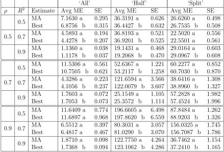
Table 3.1: Average model error and standard errors over 500 independent data sets, sample size n = 20, for the Mallows model averaged ridge regression estimates (MA) and the corresponding minimum CL model estimate (Best). Estimates found are model averaged over 100 equally spaced points over the degrees of freedom. Letters indicate groups of significantly different estimates.

‘All’ ‘Half’ ‘Split’

ρ R2 _Estimate _{Avg ME} _SE _{Avg ME} _SE _{Avg ME} _SE

0.5

0.5 MA 7.1630 a 0.295 36.3191 a 0.626 26.6260 a 0.498 Best 6.8756 b 0.315 36.4427 b 0.632 26.7535 b 0.508 0.7 MA 4.5893 a 0.194 36.8193 a 0.521 22.5020 a 0.556 Best 4.4278 b 0.207 36.9201 b 0.525 22.5501 a 0.561 0.9 MA 1.1360 a 0.038 19.1431 a 0.468 29.0164 a 0.603 Best 1.1178 b 0.037 19.2068 b 0.470 29.0967 b 0.608

0.7

0.5 MA 11.5306 a 0.561 52.6367 a 1.221 60.2277 a 0.852 Best 10.7505 b 0.621 53.2117 b 1.258 60.7030 b 0.870 0.7 MA 4.3286 a 0.223 121.6594 a 3.566 38.6416 a 1.308 Best 4.1056 b 0.237 122.0079 b 3.607 38.8960 b 1.327 0.9 MA 1.7603 a 0.072 25.1549 a 1.105 57.2828 a 1.982 Best 1.7053 b 0.073 25.3572 b 1.114 57.4524 b 1.996

0.9

(61)

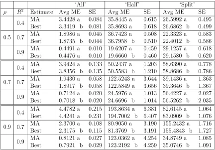
Table 3.2: Average model error and standard errors over 500 independent data sets, sample size n = 50, for the Mallows model averaged ridge regression estimates (MA) and the corresponding minimum CL model estimate (Best). Estimates found are model averaged over 100 equally spaced points over the degrees of freedom. Letters indicate groups of significantly different estimates.

‘All’ ‘Half’ ‘Split’

ρ R2 _Estimate _{Avg ME} _SE _{Avg ME} _SE _{Avg ME} _SE

0.5

0.4 MA 3.4428 a 0.084 35.8445 a 0.615 26.5992 a 0.495 Best 3.3419 b 0.081 35.8693 a 0.618 26.6862 b 0.499 0.7 MA 1.8986 a 0.045 36.7423 a 0.508 22.3323 a 0.583 Best 1.8735 b 0.044 36.7958 b 0.510 22.4012 b 0.586 0.9 MA 0.4491 a 0.010 19.6207 a 0.459 29.1257 a 0.618 Best 0.4476 a 0.010 19.6660 b 0.460 29.1580 b 0.620

0.7

0.4 MA 3.9424 a 0.133 50.2437 a 1.203 58.6390 a 0.778 Best 3.8356 b 0.135 50.5583 b 1.210 58.8686 b 0.786 0.7 MA 1.9430 a 0.058 122.5243 a 3.644 39.1436 a 1.363 Best 1.8917 b 0.058 122.5849 a 3.656 39.3646 b 1.367 0.9 MA 0.7124 a 0.020 24.5976 a 1.013 56.4227 a 2.027 Best 0.7018 b 0.020 24.6696 b 1.014 56.5262 b 2.035

0.9

Methods to Improve Prediction Accuracy under Structural Constraints.

ABSTRACT

DEDICATION

BIOGRAPHY

ACKNOWLEDGEMENTS

TABLE OF CONTENTS

LIST OF TABLES

LIST OF FIGURES

Chapter 1

Introduction

1.1

Regularization Framework

1.2

Plan of Dissertation

Chapter 2

Introduction to Model Averaging

2.1

Bayesian Model Averaging Review

2.1.1

The BMA Framework

2.2

Frequentist Model Averaging Review

2.2.1

Information Theory Weights

2.2.2

Bootstrap Weights

2.2.3

Cross Validation Weights

2.2.4

Mallows Criterion Weights

Chapter 3

Model Averaged Ridge Regression

3.1

Introduction and Motivation

3.2

FMA Review - Basic Paradigm

3.3

Adapting FMA to Ridge Regression

3.4

Weight Choice

3.4.1

Fixed Weights

3.4.2

Adaptive Weights

3.5

Model Averaged Ridge Regression using

Mal-lows Criterion

3.6

Bayesian Connection

3.7

Asymptotic Properties

3.8

Simulation Studies

3.8.1

Set-up and Competitors

3.8.2

Results

3.9

Real Data Examples

3.9.1

Pakistani Economic Data

3.9.2

Longley’s Economic Data

3.9.3

Boston Housing Data

3.10

Discussion