GENETICS | GENOMIC SELECTION
Quality Control of Genotypes Using Heritability
Estimates of Gene Content at the Marker
Natalia S. Forneris,*,††Andres Legarra,†,‡,1Zulma G. Vitezica,†,‡Shogo Tsuruta,§Ignacio Aguilar,**
Ignacy Misztal,§and Rodolfo J. C. Cantet*,††
*Departamento de Producción Animal, Facultad de Agronomía, Universidad de Buenos Aires, C1417DSE Buenos Aires, Argentina,
†INRA, Génétique, Physiologie et Systèmes d’Elevage, F-31326 Castanet-Tolosan, France,‡Université de Toulouse, INP, ENSAT,
Génétique, Physiologie et Systèmes d’Elevage, F-31326 Castanet-Tolosan, France,§Animal and Dairy Science, University of Georgia, Athens, Georgia 30602, **Instituto Nacional de Investigación Agropecuaria, Canelones 90200, Uruguay,††Consejo Nacional de Investigaciones Científicas y Técnicas, Av. Rivadavia 1917, C1033AAJ Buenos Aires, Argentina
ABSTRACTQuality controlfiltering of single-nucleotide polymorphisms (SNPs) is a key step when analyzing genomic data. Here we present a practical method to identify low-quality SNPs, meaning markers whose genotypes are wrongly assigned for a large proportion of individuals, by estimating the heritability of gene content at each marker, where gene content is the number of copies of a particular reference allele in a genotype of an animal (0, 1, or 2). If there is no mutation at the marker, gene content has an additive heritability of 1 by construction. The method uses restricted maximum likelihood (REML) to estimate heritability of gene content at each SNP and also builds a likelihood-ratio test statistic to test for zero error variance in genotyping. As a by-product, estimates of the allele frequencies of markers at the base population are obtained. Using simulated data with 10% permutation error (4% actual error) in genotyping, the method had a specificity of 0.96 (4% of correct markers are rejected) and a sensitivity of 0.99 (1% of wrong markers are accepted) if markers with heritability lower than 0.975 are discarded. Checking of Mendelian errors resulted in a lower sensitivity (0.84) for the same simulation. The proposed method is further illustrated with a real data set with genotypes from 3534 animals genotyped for 50,433 markers from the Illumina PorcineSNP60 chip and a pedigree of 6473 individuals; those markers underwent very little quality control. A total of 4099 markers withP-values lower than 0.01 were discarded based on our method, with associated estimates of heritability as low as 0.12. Contrary to other techniques, our method uses all information in the population simulta-neously, can be used in any population with markers and pedigree recordings, and is simple to implement using standard software for REML estimation. Scripts for its use are provided.
KEYWORDSgene content; quality control; SNP; genomic selection; REML; shared data resource; GenPred
I
N PLANT and animal genetics, a large number of platforms for genotyping of single-nucleotide polymorphisms (SNPs) have appeared in recent years, in addition to the use of techniques to impute from low-density to high-density chips. However, these techniques are not without technical failures. Errors in genotypes can be due to wet laboratory errors (poor DNA samples, poor readings, etc.), different biochemistry in marker panels, label switching, or mistakes in pedigree record-ing. For example, Wigganset al.(2012) removed 127 mark-ers out of 2886 in the Bovine3K BeadChip (Illumina, Inc.,San Diego, CA) because they showed.2% Mendelian con-flicts. Errors also can arise from imputation procedures; for instance, if a marker is erroneously located in the map, its flanking markers will be wrong, as will be the imputation analysis (Hickeyet al.2012; Wanget al.2013). The quality of genotypic data in genomic evaluations thus has been carefully considered for some time, and a number of proce-dures for quality control (QC) have been developed. The QC filtering of SNPs in genomic evaluation can increase accu-racy, reduce computational effort, and improve stability of es-timates of the effects of the remaining SNPs (Wigganset al.
2009). We propose a method based on maximum likelihood to check the quality of marker genotypings in a possibly com-plex pedigreed population that is partially or completely geno-typed for a set of biallelic markers. This method specifically aims at detecting loci for which a large number of indi-viduals are wrongly genotyped. First, we briefly describe Copyright © 2015 by the Genetics Society of America
doi: 10.1534/genetics.114.173559
Manuscript received September 26, 2014; accepted for publication December 18, 2014; published Early Online January 6, 2015.
Supporting information is available online athttp://www.genetics.org/lookup/suppl/ doi:10.1534/genetics.114.173559/-/DC1
current methods. Then the method is presented, and results using publicly available and simulated data are shown.
Quality Control of Genotypes
The most commonly used QCfilters include QC on individ-uals for call rate, duplicates, and parent-progeny conflicts and QC on SNPs for call rate, minor allele frequency (MAF), departure from Hardy-Weinberg equilibrium, and in partic-ular, Mendelian conflicts [see Wiggans et al.(2009) for a general description]. The latter are usually checked using data from trios and parent-offspring pairs (Wiggans et al. 2009, 2012). However, Mendelian-consistent errors usually go unde-tected (e.g., an offspringAafrom parentsAaandAAis geno-typed as AA). Another method involves checking that the progeny of one heterozygote male mated to several females has an average heterozygosity of 0.5 (Leroyet al.2013).
Cheung et al. (2014) proposed a method for detecting both inconsistent and occasionally Mendelian-consistent errors tailored to small and moderately large hu-man pedigrees (e.g., 100 subjects). While this and similar error-detection procedures are computationally efficient for detecting genotyping errors at the marker level given inferred pedigree descent patterns and may allow tracing these occa-sionally occurring genotyping errors in markers at the subject level, it is not immediately known whether this method is equally applicable to plant or livestock data that are very large in pedigree size (e.g.,.1000) and especially when the moti-vation is to detect suspicious markers in which a considerable proportion of subjects has genotyping errors.
The application of these QCfilters (except Cheunget al.
2014) does not use all available information from pedigree and markers. For instance, consider 10 full sibs, 5 with ge-notypeAAand 5 with genotypeaa, issued from both parents heterozygotes. This segregation distortion is not a Mendelian error, but it is a very unlikely situation. The problem becomes very complex for large pedigrees in which only a fraction of the animals is genotyped. For instance, VanRaden (2008) considered a pedigree with 3000 genotyped bulls, all con-nected, whose pedigree spanned 23,105 individuals.
Here we present a practical method to identify low-quality SNPs across individuals by considering gene content as a quantitative trait and testing the null hypothesish2= 1. The sensitivity and specificity of the method are evaluated by simulation of a pig breeding data set, and the method is illustrated with a real pig breeding data set.
Materials and Methods Theory of the Method
Gene content as a quantitative trait:Gene contentzat one
marker is the number of copies of a particular reference allele (e.g.,z= 0, 1, or 2 forAA,AG, andGG) (Falconer and Mackay 1996). In other words, (observed) gene content can be seen as a quantitative trait where the map of genotype to phenotype is
f0;a;2agfor the three genotypes and the additive effectaof the reference allele (Gin the preceding example) is exactly 1. Therefore, there is neither dominance nor epistasis. In addi-tion, unless there is a mutation at the marker, and if the marker is genotyped accurately, there is no error associated with the phenotype. Thus, and by construction, the heritability of gene content is 1, and all variation is strictly additive genetic. The mean of zin the base population is 2p, wherepis the allelic frequency at the base population, whereas its variance is 2pq
andq= 12p.
The covariance between both gene contents from two individuals is Covðzi;zjÞ ¼Aij2pq [Cockerham 1969, equa-tion (8)], where Aij is the additive relationship between two individuals, usually computed from pedigree [see Toro
et al.(2011) for a more detailed explanation]. This fact has been highlighted recently and used by McPeeket al.(2004) and Gengleret al.(2007) in similar contexts. Therefore, ifz contains gene content for a set of genotyped individuals, CovðzÞ ¼A222pq, whereA22is a matrix with additive rela-tionships across genotyped individuals. Moreover, A22 is a submatrix of the whole-pedigree relationship matrix A. For each marker, we may write a linear model for gene content:z¼1ð2pÞ þuþe, whereuis the deviation of each individual from this mean, andeis an error term that should be 0 in the absence of genotyping errors. In this case,s2
e ¼0 so thath2¼s2
u=ðs2uþs2eÞis equal to 1 with no genotyping errors. We recall that CovðuÞ ¼A22s2
u ands2u¼2pq.
Estimation of heritability: When analyzing complex
pedi-grees, a common method to estimate heritabilities is restricted maximum likelihood (REML) (Patterson and Thompson 1971). REML estimators were developed assuming normality, a sit-uation that does not arise for gene content, which is not a continuous trait. However, REML has optimal properties as an iterated minimum-variance quadratic unbiased esti-mator (known as MIVQUE), which has minimum variance (Searle et al. 1992). The assumption of multivariate nor-mality for gene content is a rather common one (McPeek
et al. 2004; Gengleret al. 2007) and leads to a very con-venient linearization of the problem. In particular, REML algorithms have two nice features for our purposes. The
first is that they use Henderson’s mixed-model equations,
which in this case are of the form
0 B @
191 19W
W91 W9WþA21s2e s2 u 1 C A m u ¼
19z W9z
(1976) rules, which are computationally convenient with re-spect to the equations of McPeeket al.(2004) . From thefinal output, an estimate ofpis obtained as^p¼m^=2. Another esti-mate that is slightly different because of numerical maximiza-tion ofp(andq =12p) is obtained as the solutions to the equations2
u ¼2pq,i.e., 0:56
ffiffiffiffiffiffiffiffiffiffiffiffiffiffiffiffiffi
122s2 u
p
=2.
Hypothesis testing of genotyping errors:Another feature of
REML is that it computes likelihoods, from which statistic tests can be constructed. In our case, there are two hypothesis: the null hypothesis states that there are no genotyping errors, and therefore, s2
e ¼0 (or h2¼1). The alternative hypothesis allows any positive value of the error variance. A likelihood-ratio test (LRT) can be used to reject the null hypothesis as follows: under the null hypothesis of zero genotyping error variance, the LRT statistic is asymptotically distributed as 1/2x2(0) + 1/2x2(1) (Self and Liang 1987; Visscher 2006).
P-values for the observed LRT statistic can be calculated as-suming this distribution. Although this assumes normality, LRT is known to be robust to departures from normality (e.g., Almasy and Blangero 1998).
Implementation:In practice, the method is simple. For each
marker, REML estimates ofs2
e ands2uare obtained together with the value of the maximum likelihood—this is the alter-native hypothesis. Another estimate is obtained withs2
e ¼0 (in practice, set to a very small value). Later, theP-value of the LRT is computed from the two likelihoods, and a rejec-tion threshold is established based on the preceding asymp-totic distribution and a desired Type I error (in this work, 1%). We also suggest, as a less formal procedure, an inspec-tion of the estimated heritability; heritabilities lower than 1 are suspicious.
Test in absence of pedigree: If a pedigree is not available
but most markers area prioricorrectly genotyped, we sug-gest the following untested procedure:
1. After QC based on Hardy-Weinberg equilibrium, call rates, and MAF, construct a genomic relationship matrix Gusing all markers,e.g., following VanRaden (2008). 2. Test the heritability of each marker using REML
estima-tors as earlier and matrixG(this procedure is sometimes called GREML) for the covariance of gene content across individuals.
3. Discard markers rejected by the test, and iterate the pro-cedure until no more markers are removed.
This procedure assumes that most markers are correct.
Tests of the Method
Simulations:To ascertain the sensitivity (i.e., fraction of
in-correct markers that are rejected) and the specificity (i.e., fraction of correct markers that arenotrejected) of the test, we simulated data using QmSim (Sargolzaei and Schenkel 2009) following Mendelian rules—therefore, the simulated data had no errors. We considered a simplified pig nucleus
breeding program scenario with 10 autosomal chromosomes of 160 cM each and 70,000 SNPs. First, a mutation-drift equi-librium was reached in 2500 generations of random mating in a population with effective population size equal to 500 and mutation rate 231024, followed by a severe bottleneck with effective population size of 75 evolving during 30 genera-tions. Then there was selection (not described here) during 5 generations, where 20 boars were mated with 200 sows producing 2000 offspring, with a total of 10,220 animals, with complete pedigree and 5000 randomly chosen animals genotyped for 28,254 markers with MAF.0.01.
Type I error was evaluated as the number of SNPs with
P-values above the significant level of 0.01 for the heritability
test. We assessed type II error under two genotyping error scenarios by permuting both 10 and 5% of the genotypes for each SNP. Permuting the genotypes preserves minor allele frequencies and the Hardy-Weinberg equilibrium. Permuted genotypes were random for each SNP. Actually, a permuted genotype can be replaced by a correct genotype just by ran-dom, so the number of actual errors is lower than these values and a function of the allelic frequencies as follows: in Hardy-Weinberg equilibrium, a heterozygous genotype has a frequency of 2pq, and it is permuted by another hete-rozygous genotype with probability x (of being permuted) times 2pq(the frequency of another heterozygote). Extending the reasoning to the three possible genotypes, the rate of error is x½p2ð12p2Þ þ2pqð122pqÞ þq2ð12q2Þ, a quartic in the allelic frequency. Thus, the actual error is 0.625xfor a frequency of 0.5, 0.47xacross a uniform spectrum of allelic frequencies, and lower for U-shaped distributions; in our par-ticular simulation, the actual errors were 0.02 and 0.04 for the 5 and 10% permutation rates.
Data:We used a pig data set that has been made available
to the scientific community (Clevelandet al.2012). The data set consisted of 3534 animals from a single PIC nucleus pig line with genotypes from the Illumina PorcineSNP60 chip (Ramoset al.2009) with very little QC and a pedigree tracing back two generations from the genotyped animals (N= 6473). In practice, this data set should undergo Mendelian checking of parent-offspring couples to eliminate inconsistent animals; we have preferred not to do so in order to use the data set“as is.”A total of 50,433 SNPs were used in this study after filter-ing genotypes for minor allele frequency (,0.01) and the SNP call rate (,90%) and excluding SNPs on the sexual chromo-somes. The reason to exclude MAF ,0.01 is that numerical maximization of REML is unreliable in that case. For com-parison purposes, the same analysis was carried out in two extreme scenarios by randomly permuting half or all the genotypes for each SNP in the data set.
Statistical analysis: For each SNP in the data set, the
he-ritability and the LRT statistic were calculated to test for zero error variance in genotyping. The maximum residual log-likelihoods under the full (alternative hypothesis with-outa priorion the values ofs2
(null hypothesis assuming s2
e ¼0) were obtained using remlf90 (Misztal et al. 2002). Heritability of gene content was estimated for each SNP under the full model. Estimates can be carried on in parallel if needed. Because this software uses Henderson’s mixed-model equations, the reduced model had to be approximated by specifying a very small value for the residual variance,s2
e ¼0:0001. The advantage of com-puting in this way is that standard REML software can be used. We also used QC checking based on Mendelian errors included in preGSf90 (Aguilar et al. 2014); a marker was rejected if its genotypes showed Mendelian inconsistencies in more than 1% of the parent-offspring couples or trios.
The complete scripts for QC, the PIC data set, and the three simulated data sets are available at http://genoweb.
toulouse.inra.fr/~alegarra/qualitycontrol.tar.gz. A version
with the scripts and a small subset of the PIC data set is available as Supporting Information,File S1.
Results Simulations
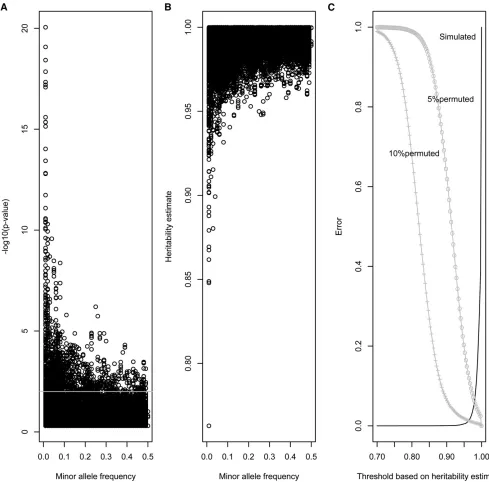
Figure 1B displays estimates of heritability (Figure 1A shows
P-value of the LRT) as a function of minor allele frequency for the data simulated with no error. Most heritability esti-mates are very close to 1, even for very low MAF values, although there is a trend that markers with very low MAF values have lower heritabilities (e.g., they may becomefixed by drift). Using a threshold at nominal 0.01 type I error, the sensitivity when 10% (5%) of the simulated genotypes were erroneous (permuted at random) was 0.99 (0.91). The spec-ificity was 0.95 (i.e., 5% of correct SNPs were rejected). Alternatively, we bounded the estimates of heritability for rejection. Figure 1C shows type I (or 1-specificity) and type II (1-sensitivity) errors against putative thresholds for rejec-tion based on heritability. For instance, if markers are rejected if their heritability estimate is lower than 0.975, this results in a specificity of 0.96 (4% of correct markers are rejected) and a sensitivity of 0.99 (for 10% of permuted data, 1% of all wrong markers are accepted). Choosing a lower bound such as 0.90 results in only 0.04% of markers being incorrectly rejected but as much as 6.5% of markers being incorrectly accepted. Thesefigures change with the level of quality, and the situation with 5% permutation of genotypes gives higher type II error. Checking Mendelian errors with preGSf90 performed worse, with 0 type I error (as expected) and 0.54 (0.84) sensitivity in the scenario where 5% (10%) genotypes were permuted. A receiving operator curve detailing results for no errorvs.10% error is available inFigure S1.
Real Data
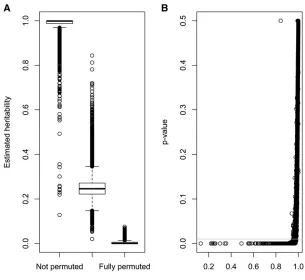
Figure 2A shows box plots for the estimated heritability of the SNPs for the original data set, the half-permuted data set, and the completely permuted data set. The original data set had a mean heritability of 0.99, and 75% of the SNPs had heritabilities above this value, although some of the markers
deviated highly from 1. When half the genotypes for each SNP were randomly permuted, heritability ranged from 0.02 to 0.84, the mean heritability was 0.25, and 75% of the estimates were below 0.27. For the fully permuted data set, all heritabilities were below 0.07. The boxes shift upward as the overall quality of the data set improves. When testing the null hypothesis of zero genotyping error ata= 0.01, the null hypothesis was rejected in 8% (N= 4099) of the SNPs of the original data set, whereas all the P-values were below 10212for the half-permuted data set and below 10293 for the fully permuted data set. The latter exemplifies how a geno-typing procedure that is largely wrong for a large percentage of the individuals (.50%) can be easily spotted using our method. The 4099 markers that did not pass the test in the original data set should be declared wrongly genotyped, and their genotypes should not be used in later analyses. Figure 2B illustrates the relationship between heritability estimates and P-values of the LRT when REML is used to estimate variance components of the original data set. It can be seen that rejected SNPs had the lower estimates of heritability, although the range of values was large (0.13, h2 ,0.97 for SNPs withP,0.01). For example, a marker with a (very) low MAF can result in high estimates of heritability, but the LRT may be inconclusive because there is very little informa-tion in the data. In general, however, using either a formal LRT or estimates of heritability will produce similar results. Using heritability estimates is less formal statistically, but it is easy to interpret for quantitative geneticists, and it can lead to an easy speed-up of the method, as discussed later. In this data set, preGSf90 checking of Mendelian errors detected only one wrong marker at 1% tolerance for Mendelian incon-sistencies, 577 at 0.1% tolerance, and 2019 at zero tolerance. Among the 577 markers with.0.1% conflicts, 388 were in common with the 4099 rejected by the heritability test. The 577 markers with .0.1% Mendelian inconsistencies had lower heritability estimates (0.92 on average) than those that were not rejected (0.99).
Discussion
correct Mendelian errors for markers that are not rejected, and in this case, the use of parent-offspring comparisons is necessary.
The method assumes a single population in Hardy-Weinberg equilibrium. The latter hypothesis seems not very restrictive because the simulated data included selection. If the population has different origins, still,s2
e ¼0. However, the hypothesis of common means and variances will not hold. An approximate method consists offitting different origins using an unknown parent groups model (Quaas 1988),i.e., allowing for different
allelic frequencies at different base populations. This assumes the same value ofs2
u¼2pqacross all populations, which will be true if the frequencies are similar across populations but will be false if there is a large divergence.
While REML estimation of heritability for a single SNP is likely to be fast, the total number of computations for a large number of SNPs can take days. In expectation-maximization REML (EM-REML), the most expensive operations in one round of iteration include (1) setting the mixed-model equations, (2) calculating solutions, and (3) calculating traces. However, the
mixed-model equations are the same for a value of heritability in all markers. Thus, dramatic costs savings can be realized when factorizations and traces are precomputed for several values of heritability. If the purpose of QC is to select SNPs with, say,h2.0.98, only three sets of such matrices would be re-quired,e.g., ath2= 0.99, 0.98, and 0.97.
Our procedure cannot identify pedigree errors (i.e., mis-labeling of DNA samples). In this case, errors are across markers in one individual instead of being across individuals for one marker. Parent-offspring discordances canflag such an error if many markers do not follow Mendelian rules for a given parent-offspring pair. There are procedures to assign parents (Wiggans et al.2009; Hayes 2011; VanRaden et al.
2013). However, a general procedure to identify and correct pedigree errors does not exist yet. A practical procedure is to compare genomic relationships (VanRaden 2008) and pedigree relationships and inspect the differences, which depend on the relationship itself and the genome architecture. A thorough de-scription of such differences can be found in Wanget al.(2014). A particular case is the use of genotypes from different chips or panels, possibly with different chemistry,e.g., the 50K and 3K panels in cattle (Wigganset al., 2012). These authors found that some markers were correctly read using one panel but not the other. In our method, this would be observed because heritability estimated including genotypes from the faulty chip, either alone or combined with the other panel, would decrease. This also applies to samples genotyped in batches;e.g., if there is a (large) batch of individual samples with poor DNA condi-tions, the addition of genotypes from the sample will decrease heritability estimates.
In our experience, this procedure is most useful when dealing with new complete data sets, in particular, from experimental studies. Regular genetic evaluations, as in dairy cattle, keep a better track of DNA samples, and because of the abundance of parent-offspring couples and trios, poor-quality markers are easily found (Wigganset al.2009, 2012).
Conclusion
We have introduced a practical QC procedure to identify SNPs with low quality across many individuals. The proposed filter is in essence an estimate of heritability of gene content at the SNPs, where any deviation from 1 is suspicious, and the
P-value is for testing the null hypothesis of“no error in geno-typing.”This QC procedure can jointly consider all geno-typed individuals and their pedigree and uses standard hypothesis-testing procedures. It should be used as a comple-ment to standard QC procedures and possibly after them.
Acknowledgments
The editor and reviewers are acknowledged for very useful comments. This work was made possible by a visit of NS Forneris to INRA, Toulouse, France,financed by the Saint-Exupéry Scholarship Program 2013–2014 (MinCyT Argentina– French Embassy). AL and ZGV acknowledge financing from projects X-Gen and GenSSeq of INRA metaprogram SelGen. NSF and RJCC were partially funded by grants UBACyT 861/2011 and PIP CONICET 833/2013. This project was partly supported by the Toulouse Midi-Pyrénées bioinfor-matics platform.
Literature Cited
Aguilar, I., I. Misztal, S. Tsuruta, A. Legarra, and H. Wang, 2014 PREGSF90–POSTGSF90: computational tools for the im-plementation of single-step genomic selection and genome-wide association with ungenotyped individuals in BLUPF90 pro-grams, in Proceedings of the 10th World Congress on Genetics Applied to Livestock Production, poster 680. American Society of Animal Science, Champaign, IL.
Almasy, L., and J. Blangero, 1998 Multipoint quantitative-trait linkage analysis in general pedigrees. Am. J. Hum. Genet. 62: 1198–1211.
Cheung, C. Y., E. A. Thompson, and E. M. Wijsman, 2014 Detection of Mendelian consistent genotyping errors in pedigrees. Genet. Epidemiol. 38: 291–299.
Cleveland, M. A., J. M. Hickey, and S. Forni, 2012 A common dataset for genomic analysis of livestock populations. G3 2: 429–435.
Cockerham, C. C., 1969 Variance of gene frequencies. Evolution 23: 72–84.
Falconer, D. S., and T. F. C. Mackay, 1996 Introduction to quanti-tative genetics, Longman, New York.
Gengler, N., P. Mayeres, and M. Szydlowski, 2007 A simple method to approximate gene content in large pedigree popula-tions: application to the myostatin gene in dual-purpose Belgian Blue cattle. Animal 1: 21–28.
Hayes, B., 2011 Technical note: efficient parentage assignment and pedigree reconstruction with dense single nucleotide poly-morphism data. J. Dairy Sci. 94: 2114–2117.
Henderson, C. R., 1976 A simple method for computing the in-verse of a numerator relationship matrix used in prediction of breeding values. Biometrics 32: 69–83.
Henderson, C. R., 1977 Best linear unbiased prediction of breeding values not in the model for records. J. Dairy Sci. 60: 783–787. Hickey, J. M., J. Crossa, R. Babu, and G. de los Campos,
2012 Factors affecting the accuracy of genotype imputation in populations from several maize breeding programs. Crop Sci. 52: 654–663.
LeRoy, P., J. M. Elsen, H. Gilbert, C. R. Moreno, A. Legarraet al., 2013 QTLMap 0.9.6 user’s manual. Available at:http://www. inra.fr/qtlmap
McPeek, M. S., X. Wu, and C. Ober, 2004 Best linear unbiased allele-frequency estimation in complex pedigrees. Biometrics 60: 359–367.
Misztal, I., S. Tsuruta, T. Strabel, B. Auvray, T. Druet et al., 2002 BLUPF90 and related programs (BGF90), CD-ROM,
Communication No. 28–07, 7th World Congress on Genetics Applied to Livestock Production, Montpellier, France.
Patterson, H., and R. Thompson, 1971 Recovery of inter-block in-formation when block sizes are unequal. Biometrika 58: 545–554. Quaas, R. L., 1988 Additive genetic model with groups and
rela-tionships. J. Dairy Sci. 71: 1338–1345.
Ramos, A. M., R. P. Crooijmans, N. A. Affara, A. J. Amaral, A. L. Archibaldet al., 2009 Design of a high density SNP genotyping assay in the pig using SNPs identified and characterized by next generation sequencing technology. PLoS ONE 4: e6524. Sargolzaei, M., and F. S. Schenkel, 2009 QMSim: a large-scale
genome simulator for livestock. Bioinformatics 25: 680–681. Searle, S. R., G. Casella, and C. E. McCulloch, 1992 Variance
components, John Wiley & Sons, New York.
Self, S. G., and K.-Y. Liang, 1987 Asymptotic properties of maxi-mum likelihood estimators and likelihood ratio tests under non-standard conditions. J. Am. Stat. Assoc. 82: 605–610.
Toro, M. Á., L. A. García-Cortés, and A. Legarra, 2011 A note on the rationale for estimating genealogical coancestry from mo-lecular markers. Genet. Sel. Evol. 43: 1–10.
VanRaden, P. M., 2008 Efficient methods to compute genomic predictions. J. Dairy Sci. 91: 4414–4423.
VanRaden, P., T. Cooper, G. Wiggans, J. O’Connell, and L. Bacheller, 2013 Confirmation and discovery of maternal grandsires and great-grandsires in dairy cattle. J. Dairy Sci. 96: 1874–1879. Visscher, P. M., 2006 A note on the asymptotic distribution of
likelihood ratio tests to test variance components. Twin Res. Hum. Genet. 9: 490–495.
Wang, C., D. Habier, B. Peiris, A. Wolc, A. Kranis et al., 2013 Accuracy of genomic prediction using an evenly spaced, low-density single nucleotide polymorphism panel in broiler chickens. Poult. Sci. 92: 1712–1723.
Wang, H., I. Misztal, and A. Legarra, 2014 Differences between genomic-based and pedigree-based relationships in a chicken population, as a function of quality control and pedigree links among individuals. J. Anim. Breed. Genet. 131: 445–451. Wiggans, G. R., T. A. Cooper, P. M. VanRaden, K. M. Olson, and
M. E. Tooker, 2012 Use of the Illumina Bovine3K BeadChip in dairy genomic evaluation. J. Dairy Sci. 95: 1552–1558. Wiggans, G. R., T. S. Sonstegard, P. M. VanRaden, L. K. Matukumalli,
R. D. Schnabelet al., 2009 Selection of single-nucleotide poly-morphisms and quality of genotypes used in genomic evaluation of dairy cattle in the United States and Canada. J. Dairy Sci. 92: 3431–3436.
GENETICS
Supporting Information
http://www.genetics.org/lookup/suppl/doi:10.1534/genetics.114.173559/-/DC1
Quality Control of Genotypes Using Heritability
Estimates of Gene Content at the Marker
Natalia S. Forneris, Andres Legarra, Zulma G. Vitezica, Shogo Tsuruta, Ignacio Aguilar, Ignacy Misztal, and Rodolfo J. C. Cantet
Figure S1 ROC curve for detection of genotyping errors. This particular ROC curve uses heritability as the rejection criteria
and combines results of “good” markers (simulation with no errors) and “bad” markers (simulation with 10% error).
Created with R package “Epi”.
0.0
0.2
0.4
0.6
0.8
1.0
0.
0
0
.2
0.
4
0
.6
0.
8
1
.0
1-Specificity
S
e
n
s
it
iv
it
y
955
Model: cc$test ~ cc$h2 Variable est. (s.e.) (Intercept) -100.504 (1.754) test 105.714 (1.804)
Area under the curve: 0.997 Sens: 99.4%
File S1
Scripts for quality control
File qualitycontrol_reduced.tar.gz containing scripts and a small example is available for download at