University of Windsor
University of Windsor
Scholarship at UWindsor
Scholarship at UWindsor
Electronic Theses and Dissertations
Theses, Dissertations, and Major Papers
2009
Rate of growth and dissipation of queue on freeways and its
Rate of growth and dissipation of queue on freeways and its
effect on crash likelihood
effect on crash likelihood
Steven Volpatti
University of Windsor
Follow this and additional works at: https://scholar.uwindsor.ca/etd
Recommended Citation
Recommended Citation
Volpatti, Steven, "Rate of growth and dissipation of queue on freeways and its effect on crash likelihood"
(2009). Electronic Theses and Dissertations. 8231.
https://scholar.uwindsor.ca/etd/8231
RATE OF GROWTH AND DISSIPATION OF QUEUE ON FREEWAYS
AND ITS EFFECT ON CRASH LIKELIHOOD
By
Steven Volpatti
A Thesis
Submitted to the Faculty of Graduate Studies through Civil
and Environmental Engineering in Partial Fulfillment
of the Requirements for the Degree of
Master of Applied Science at the
University of Windsor
Windsor, Ontario, Canada
2009
1*1
Library and Archives
Canada
Published Heritage
Branch
395 Wellington Street
OttawaONK1A0N4
Canada
Bibliotheque et
Archives Canada
Direction du
Patrimoine de I'edition
395, rue Wellington
Ottawa ON MAOISM
Canada
Your We Votre reference ISBN: 978-0-494-57632-8 Our file Notre r€f6rence ISBN: 978-0-494-57632-8
NOTICE:
AVIS:
The author has granted a
non-exclusive license allowing Library and
Archives Canada to reproduce,
publish, archive, preserve, conserve,
communicate to the public by
telecommunication or on the Internet,
loan, distribute and sell theses
worldwide, for commercial or
non-commercial purposes, in microform,
paper, electronic and/or any other
formats.
L'auteur a accorde une licence non exclusive
permettant a la Bibliotheque et Archives
Canada de reproduce, publier, archiver,
sauvegarder, conserver, transmettre au public
par telecommunication ou par I'lnternet, prefer,
distribuer et vendre des theses partout dans le
monde, a des fins commerciales ou autres, sur
support microforme, papier, electronique et/ou
autres formats.
The author retains copyright
ownership and moral rights in this
thesis. Neither the thesis nor
substantial extracts from it may be
printed or otherwise reproduced
without the author's permission.
L'auteur conserve la propriete du droit d'auteur
et des droits moraux qui protege cette these. Ni
la these ni des extraits substantiels de celle-ci
ne doivent etre imprimes ou autrement
reproduits sans son autorisation.
In compliance with the Canadian
Privacy Act some supporting forms
may have been removed from this
thesis.
Conformement a la loi canadienne sur la
protection de la vie privee, quelques
formulaires secondaires ont ete enleves de
cette these.
While these forms may be included
in the document page count, their
removal does not represent any loss
of content from the thesis.
Bien que ces formulaires aient inclus dans
la pagination, il n'y aura aucun contenu
manquant.
DECLARATION OF PREVIOUS PUBLICATION
This thesis includes material from one original paper that has been previously submitted for
publication in a peer reviewed journal, as follows:
Lee, C. and Volpatti, S. (2009). Effects of Shock Waves on Freeway Crash Likelihood. Submitted
for presentation at the 89th Transportation Research Board Annual Meeting and publication in
the Transportation Research Record. Washington, D.C., 19 pages.
I certify that I have obtained a written permission from the copyright owner(s) to
include the above published material(s) in my thesis. I certify that the above material describes
work completed during my registration as graduate student at the University of Windsor.
I declare that, to the best of my knowledge, my thesis does not infringe upon anyone's
copyright nor violate any proprietary rights and that any ideas, techniques, quotations, or any
other material from the work of other people included in my thesis, published or otherwise, are
fully acknowledged in accordance with the standard referencing practices. Furthermore, to the
extent that I have included copyrighted material that surpasses the bounds of fair dealing within
the meaning of the Canada Copyright Act, I certify that I have obtained a written permission
from the copyright owner(s) to include such material(s) in my thesis.
I declare that this is a true copy of my thesis, including any final revisions, as approved
by my thesis committee and the Graduate Studies office, and that this thesis has not been
submitted for a higher degree to any other University or Institution.
ABSTRACT
To improve traffic safety on freeways, many traffic researchers have used real time data to
predict the likelihood of crashes, using number of crashes as the measure of safety. The
parameters of speed, volume or density have been used extensively in previous research to
calculate the crash likelihood.
This research studied the combined effects of volume and density t o predict crash
likelihood using real time data a short time before crash occurrence. The volume-density
relationship provided a measure of growth and dissipation of queue on the freeway, known
as the shock wave speed. Using this shock wave speed and quantifying various types of
shock waves, analysis was done to predict crash likelihood.
The results of logistic regression analysis indicated that increasing the speed of forward
shock wave decrease crash likelihood. Using a log-linear relationship and including
exposure measures, it was found that diverging sections, normal weather conditions, low shock
wave speeds and forward moving shock waves indicated increased likelihood of crashes. Finally,
using an odds ratio t o compare the combined effects of shock wave speed and shock wave type,
it was determined that forward moving shock waves yield a greater likelihood of crash for both
To my parents, Faustino and Franca Volpatti and my sisters Angela and Diana
ACKNOWLEDGEMENTS
I would like to take this opportunity to sincerely thank my supervisor, Dr. Chris Lee, for his
continued support, assistance, guidance, and constructive evaluations throughout the course of
my thesis project. I truly appreciate the confidence he has shown in me and have learned a
great deal working with him. I would also like to thank my evaluation committee of Dr. Faouzi
Ghrib, Dr. Guoquing Zhang, Dr. Sreekanta Das and special committee member, Mr. John
Tofflemire, for their suggestions to improve this thesis. I would like to send a special thank you
to Mr. Tofflemire, who introduced me to traffic and transportation engineering.
I would also like to express thanks to my friends as well as colleagues at the University,
especially Benjamin Hodi, Thomas Ring, Sara Kenno, Adam Mourad and James Bryant, who have
lent their support and expertise throughout the course of this project.
A heartfelt thank you goes out to Dr. N.K. Becker. Dr. Becker first introduced me to civil
engineering and has always been available to help with any concerns I may have had throughout
my studies. He has always been supportive of me and challenged me to strive for the top.
Lastly, I would like t o thank my parents, Faustino and Franca and my two sisters, Angela and
Diana, for their continued encouragement, support and belief in me throughout the course of
TABLE OF CONTENTS
DECLARATION PREVIOUS PUBLICATION iii
ABSTRACT iv
ACKNOWLEDGEMENTS vi
LIST OF TABLES ix
LIST OF FIGURES x
NOMENCLATURE xi
1 INTRODUCTION 1
1.1 Overview 1
1.2 Research Objectives 2
1.3 Organization of Thesis 2
2 LITERATURE REVIEW 3
2.1 Traffic Flow Theory 3
2.2 Shock wave Theory 7
2.3 Real-Time Crash Analysis 8
2.4 Evaluation of Literature 12
3 DATA 14
3.1 Traffic Data 14
3.2 Incident Logs 15
3.3 Weather Data 16
3.4 Exposure 17
4 PROCEDURE 19
4.1 Classification of Shock waves 19
4.2 Critical Values and Trends 20
4.3 Determining Shock wave 24
4.4 Effect of Ramps on Mainline Traffic 27
4.5 Statistical Analysis Techniques 27
4.5.1 Logistic Regression Model 28
4.5.2 Log Linear Model 28
5 RESULTS AND ANALYSIS 32
5.1 Shockwaves 32
5.2 Effect of Ramps on Mainline Traffic 40
5.3 Ideal Time Period 41
5.4 Logistic Regression Model 41
5.5 Log linear Model 43
6 CONCLUSIONS AND RECOMMENDATIONS 50
6.1 Conclusions 50
6.2 Recommendations 51
REFERENCES 53
APPENDIX A 55
LIST OF TABLES
Table 3-1: Sample Raw Data 15
Table 3-2: Exposure for Each Road Section 18
Table 5-1: Shock waves Sorted by Shock wave Type (Crash Cases) 32
Table 5-2: Average Shock wave Speed by Type (Crash Cases) 34
Table 5-3: Shock waves by Shock wave Type (Non-Crash Cases) 35
Table 5-4: Average Shock wave Speed by Type (Non-Crash Cases) 37
Table 5-5: Results of Log Linear Model - Eastbound Lanes 45
Table 5-6: Results of Log Linear Model - Westbound Lanes 46
Table 5-7: Observed and Expected Frequencies 47
Table 5-8: Exposure Comparison-Westbound Lanes 48
Table 5-9: Log-odds Ratio - Westbound Lanes 49
LIST OF FIGURES
Figure 2.1: Time Space Diagram of Vehicle Trajectory 4
Figure 2.2: Volume-Density Relationship 5
Figure 2.3: Speed-Volume Relationship 6
Figure 2.4: Speed-Density Relationship 7
Figure 2.5: Calculating Shock Wave Speed 8
Figure 3.1: Detector Location on the Gardiner Expressway 14
Figure 3.2: Speed Profile - Station 60 16
Figure 4.1: Shock wave Types 20
Figure 4.2: Volume-Density Graphs for Westbound Traffic 22
Figure 4.3 : Volume-Density Graphs for Eastbound Traffic 23
Figure 4.4: Shock wave Types 26
Figure 4.5: Averaging Points 27
Figure 5.1: Frequency of Crashes 38
Figure 5.2: Frequency of Crashes-Forward Shockwaves , 39
Figure 5.3: Frequency of Crashes- Backward Shock waves 40
exp
F„
Fij
k
ni
P.(k)
P ( Y = i )
q
NOMENCLATURE
exposure (log-linear model)
expected frequency for variable A with category i and variable B with category j (log-linear model)
expected frequency of case (Log odds ratio)
expected frequency of base case (Log odds ratio)
density of road section (veh/km)
observed frequency (Chi-Square Statistic) —
probability that frequency of event is (k=0, 1, 2, 3,...) - (Poisson)
the probability of occurrence of a crash (logistic regression model)
volume of road section (veh/hr)
ShockSpeed actual shock wave speed in km/hr
t number of intervals (Poisson)
u speed (km/hr)
xik explanatory variable (logistic regression model)
Y-, random variable of accident counts on entity i (Negative Binomial)
y, specific accident count on entity j (Negative Binomial)
a constant (logistic regression model)
fa coefficient for the explanatory variable (logistic regression model)
pexp coefficient o f t h e exposure measure (log-linear m o d e l )
q, expected n u m b e r o f events (Negative Binomial)
6 c o n s t a n t (Log odds ratio)
A, e x p e c t e d value o f e v e n t f r e q u e n c y f o r ith interval (Poisson)
AGEOMETRV coefficient f o r g e o m e t r i c c o n d i t i o n (log linear m o d e l )
^WEATHER coefficient for weather (log linear model)
^SHOCKTYPE coefficient for shock wave type (log linear model)
ASHOCKSPEED coefficient f o r shock w a v e speed (log linear m o d e l )
^TYPESPEED coefficient f o r i n t e r a c t i o n b e t w e e n shock w a v e t y p e a n d shock w a v e speed ( l o g linear m o d e l )
K[\), Ayp) coefficients f o r variables X and Y (Log odds ratio)
^xy(ii)/ ^xy(ij) coefficient f o r interaction o f variables X and Y (Log odds ratio)
Ax(D coefficient f o r base case (Log odds ratio)
Hj e x p e c t e d f r e q u e n c y (Chi-Square Statistic)
4> overdispersion parameter (Negative Binomial)
X chi-squared statistic
1 INTRODUCTION
1.1 Overview
Over the last half century, the transportation industry has become an essential need for many
people around the world, especially in North America, whether it is freight shipping for
businesses or for one's personal use to travel to and from work. Due t o increase in demand for
trips by motor vehicle, the increased capacity of road is needed. Over the years, there have
been significant advances in road design and traffic management to alleviate congestion and
improve safety for travelers. Some of the road design and traffic management methods
include-enhancing road geometric conditions such as increased lane width, increased stretches of
straight roadways, strengthened and reinforced pavements, increased and enhanced traffic
signage, and intelligent traffic control.
Prior to any additions or upgrades to the road network, studies must be conducted to determine
if there is a need for any changes, and how the changes will affect the current traffic situation in
the study area. Safety can be measured in many ways; however it is commonly measured in
terms of number and severity of crashes in the network.
Existing road networks are continually monitored by researchers and planners to identify the
locations with high number of severe crashes. In more recent years, given that crashes tend to
occur due to short term variation in traffic flow, traffic conditions have been monitored in real
time. These real-time traffic flow parameters have been related to the potential of crash
occurrence. With the adaptation of real-time traffic conditions, it is possible to predict the
dangerous conditions in advance and prevent crashes. Research is focused on proactive
approaches to prevent crashes rather than reactive measures. The goal of the research is to use
proactive approaches to determine whether or not a crash will occur based on the most up to
date traffic conditions.
1.2 Research Objectives
The goals of this research are as follows:
1. To understand how a queue forms or dissipates in a short time period before a crash
occurs.
2. To estimate the likelihood of crash occurrence - based on queue formation and
dissipation.
1.3 Organization of Thesis
The thesis is organized in six chapters. Chapter 2 deals with literature review of traffic flow
theory, shock wave theory, studies on real-time analysis of traffic data and the likelihood of
crash risk and studies indicating the effects of shock wave speed on traffic flow. Chapter 3
describes the data used in this study. Chapter 4 covers the procedure used in the study.
Chapter 5 presents results and analysis of the study. Chapter 6 includes the conclusions and
2 LITERATURE REVIEW
2.1 Traffic Flow Theory
Traffic flow theory explains interaction between vehicles and the roadway system. The theory
was developed from physics and mathematics to explain the relationships of traffic stream
parameters. Traffic stream parameters are classified as one of two broad categories:
microscopic parameters and macroscopic parameters.
Microscopic parameters reflect the behaviour of individual vehicles in a traffic stream and the
microscopic traffic flow models describe the behaviour of the car following. The parameters
used for an individual vehicle are: spacing (s), headway (h,) and speed (Ui). The spacing is
defined as the distance between two successive vehicles and has units of distance per vehicle.
The headway is defined as the time between two successive vehicles, in the units of time per
vehicle. The speed is the distance per unit time for each vehicle. The spacing, headway and
speed can be measured using a time-space diagram of vehicle trajectory. In Figure 2.1, the
spacing is the vertical distance between the vehicle's trajectories, whereas the headway is the
horizontal distance between the vehicle's trajectories. The instantaneous speed is the slope of a
line tangent to any point on the vehicle's path. The vehicle trajectories in the following figure
indicate that the vehicles are not travelling at a constant speed given that the paths are not
straight lines.
T i m e Space Diagram o f Vehicle Trajectory
Distance
Instantaneous Speed = slope
• Vehicle B
•Vehicle A
Time
Figure 2.1: Time Space Diagram of Vehicle Trajectory
Macroscopic parameters are the average behaviour of a group of vehicles. The traffic flow
models for these parameters describe the relationships among volume, speed and density.
Volume (q) is defined as the number of vehicles that pass through a given interval in a specified
period and is typically measured in vehicles per hour. Density (k) is the number of vehicles that
pass a given length of road, usually recorded in vehicles per kilometre. These three parameters
are interrelated in the following fundamental equation of traffic flow:
(1)
k = ^
Given that it is very difficult to measure the density in the field, the density is usually calculated
using this equation.
Traffic flow can be classified into two principle categories: 1) uninterrupted flow: flow of traffic
is not disrupted by external factors (e.g. freeway flows), and 2) interrupted flow: traffic flow is
disrupted periodically by external factors such as traffic signals or signage in the road network.
For uninterrupted flow, the combinations of speed, volume and density are able to produce
further two-dimensional relationships, which can be used to extract valuable information about
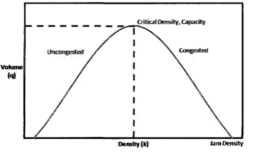
the traffic flow in the area of interest. Figure 2.2 shows the relationship between volume and
density, which forms an inverted parabolic shape. In this figure, the highest point of the
parabola in the q-axis represents the capacity and the critical density of the roadway, with all
values to the left of the point being in the uncongested state and all values to the right of this
point being in the congested state. The capacity is the point in which the road network is
considered t o have reached its maximum number of vehicles per unit time. The point where the
congested side of the parabola intersects with the k-axis is the jam density. The jam density is
the maximum number of vehicles per unit distance, which occurs when volume is zero (i.e. all
vehicles are stopped).
Volume (q)
Density (k) Jam Density
figure 2.2; Volume-Density Relationship
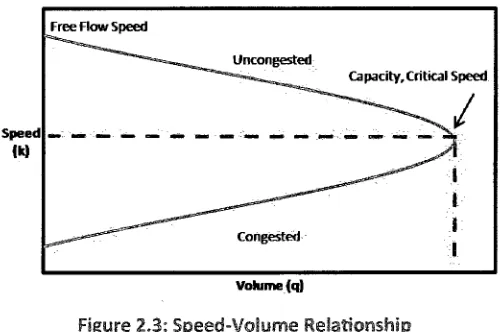
The relationship between the speed and the volume also forms a parabolic relationship as
shown in Figure 2.3. The highest point in the q-axis again represents the capacity of the
roadway, and the speed at capacity is called the critical speed. This critical speed specifies the
boundary between uncongested and congested flow. The uncongested flow is represented by
the top portion of the graph (when the speed is greater than the critical speed) whereas the Critical Density, Capacity
congested flow is represented by the lower portion of the graph (when the speed is lower than
the critical speed. The other important point from this graph is the free flow speed, which
occurs when the volume is zero and the speed is maximum (highest point on the graph). Traffic
engineers use this graph to find the level of service of a road network. The system assigns a
grade based on the traffic flow from A to F, with A being the free flow speed, progressing along
t o E, which is the critical speed and capacity, and the congested phase, represented by level of
service F. This is primarily used when determining what roads need to be upgraded within a
system when a change occurs to increase the capacity of the road (e.g. new subdivision, new
commercial centre, etc.).
Volume (q)
Figure 2.3: Speed-Volume Relationship
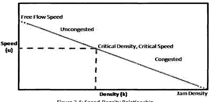
The third relationship is between speed and density is shown in Figure 2.4. The form of this may
not necessarily be a straight line, but in general, speed and density simultaneously increase and
decrease. From this graph, the free flow speed and the jam density can easily be obtained,
using the intersection points of the u-axis and k-axis respectively for the values. There exists a
transition point between uncongested and congested flow, specifically at the critical speed and
Speed
M
Free Flbw Speed
Uncontested
^Critical Density, Critical Speed
I "*****»^ - :Cbngestfed:
I
J .
Density (k)
Figure 2,4: Speed-Density Relationship
Jam Density
As shown in the previous three figures, all three traffic flow parameters are closely related to
each other. It should be noted that the volume itself cannot reflect the level of congestion due
to the fact the same volume can occur for both uncongested and congested conditions. Another
useful method of quantifying the level of congestion on the freeways is to investigate the effects
of the rate of growth and congestion of queue on freeways. This is called shock wave analysis.
2.2 Shock wave T h e o r y
Shock wave theory is a classical theory that was first derived by Richards (1956) and later
developed by Lighthill and Whitham (1957). The traffic state is represented by flow and
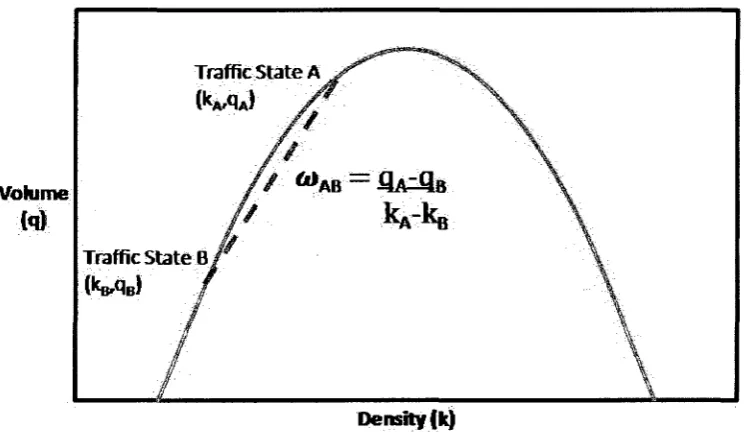
concentration of traffic (or density). Shock wave is defined as the change in volume (measured
in veh/hour) divided by the change in density (measured in veh/km) between two traffic states.
The speed of the shock wave is typically measured in km/hour. The equation of a shock wave
represents the formula for the slope of a line as follows:
(2)
Aq qA-qB
(OAB = — =
Ak kA- kB
Where,
6jAB = speed of shock wave moving from traffic state A to traffic state B;
kA, kB = densities at traffic states A and B, respectively.
Since the parameters for measuring shock wave speed are volume and density, the graphical
relationship shown in Figure 2.5 can be used to calculate the speed of the shock wave. Shock
wave theory is useful for quantifying the rate of growth or dissipation of queue.
Volume
M
Traffic State A
Traffic State B
( M B )
Density (k)
Figure 2.5: Calculating Shock Wave Speed
2.3 Real-Time Crash Analysis
To investigate the impact of traffic flow on crash likelihood, it is worthwhile to examine traffic
conditions during the short time immediately before a crash occurs. Hall et al. (1986) concluded
that real-time traffic analysis is advantageous in identifying patterns that exist on a roadway
that may not be visible when using scatter diagrams of traffic data. They also found that the
real time traffic analysis can identify transition points between congested and uncongested
Since real-time data has become readily available and easily accessed, numerous researchers in
recent years have attributed analysis of real-time traffic flow on a freeway as an important tool
for predicting crash likelihood. Oh et al. (2001) investigated the factors that contributed to
traffic accidents in real-time using probability density functions distinguishing typical and
disruptive traffic conditions, and concluded that the reduction in speed variation is crucial to
reduce accident likelihood. Lee et al. (2002) investigated real-time crash precursors of variability
on speed and traffic density on a stretch of freeway to predict potential for crashes using a log
linear model, which accounted for exposures. The results of this paper indicate that these crash
precursors are significant with controls for geometry, weather and time of day. Lee et al. (2003)
expands the previous study by re-evaluating the model and suggesting methods to determine
the crash precursors objectively and to test and compare this modified model with the previous
model. After comparing these models, it was noted that the variables could be determined
experimentally and less subjective judgment is required for determining categories of crash
precursors. Another finding from this study was that crashes were more likely to occur when
there was a significant difference in speed between a downstream and an upstream detector,
indicating that the formation and/or dissipation of traffic queue is affecting crash risk.
Golob et al. (2004) presents a strong relationship between traffic flow conditions and likelihood
of crashes. In this study, the mean volume and median speed, as well as the temporal variations
in volume and speed determined 30 minutes prior to a crash occurrence had a strong
association with the type of crash. The researchers in this study believe that identifying the type
of crash is instrumental in enhancing safety on the roadway.
Abdel-Aty et al. (2004) developed a crash likelihood prediction model using real time traffic flow
data and tested the crash identification percent. The first finding of the study was that 5 to 10
minute occupancy upstream of the crash site and the 5-minute coefficient of static variation in
speed downstream of the crash site had the greatest impact on crashes. Using these factors,
and with a threshold value of 1.0 for the log-odds ratio, 69% of the crash identification was
achieved. From this conclusion, it can also be said that real time traffic data can indeed predict
crashes. In a similar study, Songchitruksa and Balke (2006) determined that the same variables
of 5-minute average occupancy and coefficient of variation in speed are good indicators of
freeway crashes. The nested and nonnested multinomial logit models provided in this paper
demonstrated how the variables mentioned detected the probability of an incident in the next
15-minutes using the real time data. Also, by comparing crash and non-crash data, there was a
low false alarm rate. This paper also demonstrated factors other than traffic flow variables can
determine the incident type using the same logit model. These factors included, visibility,
lighting and time of day.
Pande and Abdel Aty (2005) expanded on a previous study to show the log of coefficient of
temporal variation in speed, standard deviation of volume, and average occupancy expressed as
percentage are significant in determining potential occurrence of a crash. Using these findings,
another case-controlled logistic regression model was adapted to proactively determine
whether or not a crash will occur, and using the data once again, the model was able to predict
if a crash was going t o occur in the upcoming 15 to 20 minute period. The authors also mention
they have used a general model, and to use on a specific freeway, location, geometry, day, day
of week would have to be used to calibrate the model to the particular section of freeway.
include a rain index variable, and determined along with the rain index, the 5 minute average
occupancy, the standard deviation of the volume downstream and 5 minute coefficient of
variation in speed 5-10 minutes prior to the crash had significant affects on the crash occurrence
and that it is possible to predict the likelihood of a crash prior to occurring.
A more empirical approach was studied by Hourdos et al. (2006). This study used individual
vehicle speeds and headways from video cameras and tested the relationship between real time
traffic conditions and likelihood of a crash by using only certain sections of the freeway with
crash prone conditions, by first developing a model specific for the crash prone area. The
authors also stress the importance of testing the models that are developed to test for accuracy.
The crash model yielded a 58% success rate in predicting crashes, with only a 6.8% false
detection rate. Qi et al. (2007) also presented an empirical analysis of real time traffic data to
develop an accident frequency model using time series and cross sectional measures and the
results indicated traffic flow characteristics, weather, and geometry were statistically significant
with traffic accidents. A study by Son et al. (2009) used real-time individual vehicle and crash
data similar to Hourdos et al. (2006) to determine shorter headway is more likely to contribute
t o crashes.
As mentioned in the previous section, the theory of shock waves was originally derived by
Richards (1956) and Lighthill and Whitham (1957). Since then, researchers have used different
methods to estimate shock wave speeds. Messer et al. (1976) used combined equations of the
kinematic wave model and Greenshields' macroscopic traffic flow to estimate the speeds of
shock waves formed after an incident occurs and a lane-blocking ensues. More recently, Hurdle
and Son (2000) used density contour maps containing spatial and temporal propagation of
traffic regimes with similar densities t o estimate the shock wave speeds. Expanding on the
previous paper, Hurdle and Son (2001) used three examples to demonstrate that shock waves,
arrival and departure curves for modeling freeway congestion curves are indeed compatible.
Another method of shock wave estimation by Windover and Cassidy (2001) compared
cumulative counts composed from vehicle counts. The previous two papers measured shock
waves at fixed locations in the freeways studied; however Lu and Skabardonis (2007)
determined shock waves based on individual vehicle trajectories under congested conditions.
Although these papers discuss methods to determine shock waves, none of them has related
the speed or type of shock wave to the likelihood of freeway crashes.
2,4 E¥aluation of Literature
In recent years, many studies have been conducted t o predict time crash risk using
real-time measures of speed, volume and/or density for stretches of highways. These studies work
better in predicting crashes than the studies that used average traffic data such as the annual
average daily traffic volumes (AADT). The other advantage of using real-time data is that high
crash risk can be detected in advance and crash occurrence can be potentially prevented before
the crash actually occurs. This is valuable because it should significantly reduce the number of
crashes once real time models can be implemented in traffic management systems. At the very
least, traffic management centres can be prepared for incidents that may occur using real-time
predictor models, leading t o better response times when an incident occurs, thus decreasing
wait times due to lane closures or blockages that may occur. Another important finding that has
been noted in a majority of these studies that variations in speeds between loop detector
stations is a strong indicator of crash occurrence, and the recommendations from these studies
methods such as standard deviations some time period cannot show proper growth and
dissipation effects.
Although Shockwave speeds have been studied and methods to determine speed of shock wave
are being established, there seems to be no link between this and crash likelihood methods.
With the readily available short-term aggregated loop detector data, the choice of using this
data as opposed to vehicle trajectories, as in the previous studies, needs to be investigated.
3 DATA
3.1 Traffic Data
The data for this thesis were collected through loop detector stations located on a section of the
Gardiner Expressway in Toronto, Ontario, Canada. The Gardiner Expressway is an urban
freeway, frequently used by local commuters going to and from downtown Toronto. The
studied section of the freeway analyzed has three lanes in each direction and is a fairly straight
stretch of road. The westbound section is especially important because of the Jameson Ave. on
ramp, which is closed from 3 pm to 6 pm in an attempt to alleviate congestion of the mainline
traffic. An off-ramp is located upstream of the on-ramp, where significantly higher number of
crashes occurs than other sections of the freeway (mainline station 80). The eastbound lanes
have an on-ramp and two off-ramps on the studied section. The schematic drawing of this
section of freeway is shown in Figure 3.1. Also shown in the figure are the distances between
each of the loop detectors, in metres. The closest upstream station to the crash is assumed to
be the crash location.
N o t t o Scale 120
1 1 0
Jameson Ave.
110 90
0 O 0
0" 620 <$ 660 O
^ •;. • — • . . . . — - „ . 510
O
"o"
640Distance between Stations (m)
70
0
w
4900 / O
-~OWes~tbou~nd"^>~" ~+
0
0
0
0
0
0"
0
0
0
120.
\
0
• ' < > "
o
0"
100 80
O Eastbound O
- — • - - - " — £ - •
•6.0
Loop Detectors Station
The loop detectors monitor and record the 20-second volume, occupancy and speed data in
each lane. The sections of interest were mainline stations 60, 70, 80, 90, 100, 110 and 120 for
both eastbound and westbound lanes and ramp loop detector stations 110 and 120 in the
westbound direction. For the ramp loop detector stations, only the one-lane 20-second volume
was available. A total of 114 crashes occurred in the westbound lanes and 56 crashes occurred
in the eastbound lanes for the 13-month period from January 1s t, 1998 to January 31s t, 1999. A
sample of the raw data obtained at the loop detector station 60 is shown in Table 3-1.
Tatsle 3-1: Sample Raw Data
TIME 18:00:03 18:00:23 18:00:43 18:01:03 18:01:23 18:01.43 18:02:03 18:02:23 18:02:43 SPEED (km/hr) median 37 41 44 47 49 36 29 39 43 middle 41 52 si 45 52 47 49 44 49 shoulder 54 60 59 56 56 56 56 54 58 VOLUME (weh/hr) median 2340 1800 1980 2160 2160 2340 1980 1980 1980 middle 1800 1800 1980 1980 1800 2160 1980 1800 1980 shoulder 2340 2160 1620 1620 1980 1800 2160 2340 1800 OCCUPANCY (%) median 35 25 26 27 26 38 38 29 26 middle 27 22 24 29 27 29 24 27 26 shoulder 25 22 17 19 23 19 24 25 21
3.2 Incident Logs
Data for crashes were obtained through incident logs at the City of Toronto's traffic
management centre. Every incident which blocks one or more lanes of the freeway is logged
and all of the following information is recorded: a unique ID (for cases that a crash occurred,
this was the crash ID number), date (year, month, day, day of week), station (closest upstream
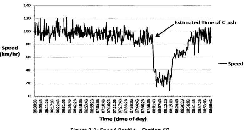
station), the reported time and the weather condition. The time of crash occurrence was
estimated based on the speed profiles using the time and speed values in each of the cases, and
was determined to be the time when the speed abruptly drops. Figure 3.2 shows an example of
the estimated time of crash at the detector station immediately upstream of the crash location.
tn'-t*> '*•>.'<*> *•> t*> *** m m m m tn m m t** t^v m .tn m t n tn tn • **> tn «** <*v «*i. m tn tn tn tn
0 ?" * " * 0 - * 0,s * r > i C D . * t > l C D ^ * rM O -si" e^ O -tT t^ CD ^T ^T r* O -^t r^ O • * rJ CD -«r CD u°) ^ 4 r^ t*t ^ t « D o * OO tn O i m O t o 0 > i r » c o C n ^ f r C D t O r - i r ^ t * > 0 » "t»" O t o * - l 1 ^ t n GO CD O f t r < C M «*> t n ^J- . * t O m C D * - « . > - t t > l t - ^ t n t n ^*- t # l 1 0 CD CD t - t t - t * X -<«» t n ^ f . * •*> " V i i i v> t o u i v> v t o t o t o t o t i i r ^ - i ^ - i - ^ i - C r ^ r ^ r ^ r ^ r ^ i - ^ c o c o c o c © 09 on do do 60 do do
CD CD O O O CD O O CD CD CD CD CD CD CD O • • O O CD CD O O CD O O CD CD O O C3
Time (time of day)
Figure 3.2; Speed Profile - Station 60
In traffic research, it is common that traffic flow conditions are distinctly different in the three
time periods of the day - morning peak, afternoon peak and an off peak groups. This is the
approach used for the eastbound traffic using a morning peak of 6 am to 9 am, an off peak
period of 9 am to 3 pm and 8 pm to 11 pm, and an afternoon peak period from 3 pm to 8 pm.
Due t o the closure of the Jameson Ave. ramp, the afternoon peak period for the westbound
lanes is further broken into two categories, afternoon peak with the ramp closed (from 3 pm to
6 pm) and afternoon peak with the ramp open (6 pm to 8 pm). The morning peak period runs
the same as the eastbound lanes from 6 am to 9 am and the off peak period goes from 9 am to 3
pm and 8 pm to 11 pm (no crashes were recorded from 11 pm to 7 am in either direction).
3.3 Weather Data
Weather data for the freeway were also obtained. Hourly weather data, provided by
Environment Canada, is labeled as either normal or adverse (rain, snow) condition each hour.
Although different adverse weather conditions lead t o different driver reactions, all of them
was considered to be normal weather conditions, and 13.2% of the time was considered to be
adverse weather conditions.
3.4 Exposure
To account for the effect of exposure on crash frequency, exposure needs to be estimated. In
traffic safety research, exposure is typically measured as the number of vehicles multiplied by
the length of the road section.
The total number of vehicles*kilometres for the 13-month period in each road section was
calculated using daily traffic volume data obtained from loop detectors, AADT was multiplied by
the length of the road section(i.e. distance between two successive loop detectors). This was
multiplied by the number of weekdays in the 13-month period since this study only considers
weekdays. The total exposures for road sections of each geometric type (straight, merging and
diverging) are summarized in Table 3-2.
Table 3-2: Exposure for Each Road Section Lane WESTBOUND EASTBOUND Detector ID dw0060dwg dvu0070dwg dw0090dwg dwOllOdwg dw0120dwg Lanes 3 3 3 3 3 Road Type straight straight straight straight straight TOTAL STRAIGHT dwOlOOdwg dw0080dwg dw0060deg dw0070deg dwOOSOdeg dw0120deg 3 3 3 3 3 3 mefging diverging straight straight straight straight TOTAL STRAIGHT dw0090deg dwOlOOdeg 3 3 merging merging TOTAL MERGING
dwOllOdeg 3 diverging AADT (veh/hr) 4,116 4,104 3,827 4,209 4,178 20,434 3,612 3,975 4,011 4,101 3,991 3,953 16,056 3,976 3,514 7/490 3,949 AADT (veh/day) 98,784 98,495 91,847 101,014 100,275 490,415 86,681 95,400 96,264 98,428 95,780 94,880 385352 95,434 84331 179,766 94,765 Distance 570
4 9 0
510
6 2 0
590
2,780
6 6 0
6 4 0
7 9 0
5 7 0
4 9 0
6 2 0
2,470
6 4 0
500
1,140
6 7 0
Total weh'km 56,307 48,263 46,842 62,629 59,162 1363354 57,209 61,056 76,049 56,104 46,932 58^26 951320 61,078 42,166 204333 63,492 Total veh*km/13-month 15,934,847 13,658312 13,256,289 17,723,943 16,742378 385329,158 16,190,205 17,278348
2 0 2 1 , 7 4 2
4 PROCEDURE
4.1 Classification of Shock waYes
There are various ways of classifying shock waves based on the movement of shock wave
between the two traffic states (A and B). This thesis classifies the shock waves based on three
criteria. The first criterion is the direction of shock wave movement. If shock wave is moving in
the same direction as the traffic flow (indicated by the positive slope of shock wave in the
volume-density curve), it is classified as a forward moving shock wave. If shock wave is moving
in the opposite direction of traffic flow (indicated by a negative slope of shock wave in the
volume-density curve), it is classified as a backward moving shock wave.
The second criterion is the growth/dissipation of congestion. If the queue is growing over time
(indicated by increasing density), the shock wave is forming. If the queue is dissipating over
time (indicated by decreasing density), the shock wave is recovering.
The third criterion is the traffic state for each point. Some shock waves occur in the same traffic
state (congested or uncongested) and some shock waves move between two traffic states
(moving from congested to uncongested or vice versa). Using these three criteria, the following
eight types of shock waves can be classified:
Type 1-1: Forward forming shock wave in uncongested region;
Type 1-2: Forward forming shock wave moving from uncongested to congested region;
Type 2-1: Forward recovery shock wave in uncongested region;
Type 2-2: Forward recovery shock wave moving from congested to uncongested region;
Type 3-1: Backward forming shock wave in the congested region;
Type 3-2: Backward forming shock wave moving from uncongested to congested region;
Type 4-1: Backward recovery shock wave in the congested region;
Type 4-2: Backward recovery shock wave moving from congested to uncongested region.
Each type of shock wave is shown graphically in Figure 4.1.
Density (k) Density (k)
(a) Forward Forming (b) Forward Recovery
Density (k) Density(k)
(c) Backward Forming (d) Backward Recovery
Figure 4 . 1 : Shock wave Types
4.2 Critical Values and Trends
Prior to analyzing data, it was required to determine the critical density and capacity values on
the freeway to identify the congested and uncongested states. To determine these values,
volume-density relationship. This was done separately for different time periods of the day
(morning peak, off peak, and afternoon peak periods) to observe the differences in traffic
patterns. It was observed from these graphs that a critical density is approximately 30 veh/km
and the roadway has a capacity of approximately 2300 veh/hour/lane.
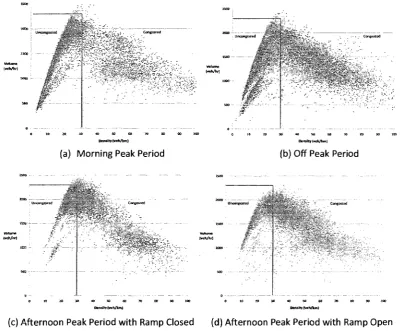
Clear differences among the time periods were observed from the graphs. In the westbound
lanes, the traffic flow conditions are split into four distinct time periods, morning peak, off peak,
afternoon peak with the ramp closed and afternoon peak with the ramp open. In the morning
peak period, more points are concentrated in the uncongested zone with fewer points in the
congested zone. In the off peak period, points are more evenly scattered in both the
uncongested zone and congested zone. In both of the afternoon peak periods, with and without
ramp closure, a majority of points are scattered in the congested zone. However, the points are
clustered around the critical density and capacity of the roadway when the ramp is closed,
whereas more points are scattered in the congested region with the ramp open, likely due t o
the severe congestion when the ramp opens. The graphs are shown in Figure 4.2.
^ ^ P P l
a t o 20 tO 50 GO
Density (vehAmj
mmm
Oenshy|veh/km)
(a) Morning Peak Period (b) Off Peak Period
m m
^
m f e
10 20 30 70 SO SO 100
Denxitvtveh/km)
0 I 0 M M B 1 M 6 0 3 O S J ) Density (vtJi/km)
(c) Afternoon Peak Period with Ramp Closed (d) Afternoon Peak Period with Ramp Open
Figure 4.2: Volume-Density Graphs for Westbound Traffic
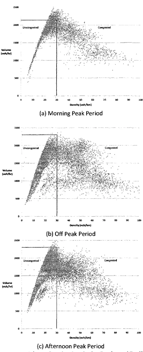
For the Eastbound traffic, only the typical three time periods were used, morning peak period,
off peak and afternoon peak period because there was no ramp closure. A strong linear trend
can be observed in the morning peak period in the uncongested zone, with a small cluster of
points in the congested zone. A similar trend was observed in the uncongested zone, but more
points are scattered in the congested zone during the off-peak period. Finally, similar
volume-density pattern was observed during the afternoon peak period. The volume-volume-density graphs for
the eastbound traffic are shown in Figure 4.3. Overall, the volume-density patterns are not
SB;
Volume fwEh/hr)
0 10 30 40 SO 60 10.
Density [weh/tan)
90 100
(a) Morning Peak Period
t _ - , - , »
a IO m M ao s o GO TO 30 100
(b) Off Peak Period
Volume £?"
S U ' W - ^ - 0 - p . w d
M M 4 O 5 O G 0 7 O 8 O 9 O . I O 0
(c) Afternoon Peak Period
Figure 4.3 : Volume-Density Graphs for Eastbound Traffic
4,3 Determining Shock wave
Once the critical density and capacity were determined from the volume-density graphs, a
volume-density curve was plotted for a ten-minute period (arbitrarily chosen) prior to the time
of crash for each crash case. Although the original data were recorded in 20-second intervals,
one-minute cumulative average data were used to account for possible random fluctuation of
values in the data. In each crash case, the presence of shock wave was checked. If shock wave
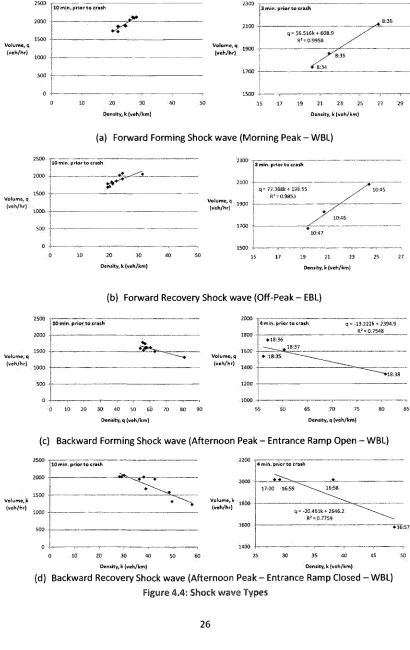
was present, the type and speed of the shock wave were measured. Shock waves were
measured in t w o ways. In the first method, if the points showed a linear trend, simple linear
regression was used t o calculate the shock wave speed as shown in Figure 4.4 three or four
minutes prior to crash time. This method was used mainly for crashes that stayed in the same
zone (uncongested or congested) since they showed linear trends. The second method was to
take an average of the cluster of points in different parts of the last ten minutes then measuring
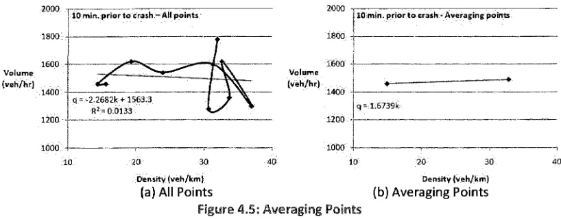
the slope of the line between the dots representing the average of the cluster of points. Figure
4.5 (a) shows no real trend of the points, but by taking the average of the clusters of the first
two points and the average of the last six points and joining the two average points, good shock
wave estimation is produced as shown in Figure 4.5 (b). This method was not used often, but
was typically used for cases that switched from uncongested zone to congested zone or vice
versa.
In the westbound lanes, there were a total of 114 crashes, with 62 cases (54%) showing a shock
wave occurrence in the last 10-minutes, and 75 cases (66%) in the last 3-10 minutes (called
"short term") prior to the crash time. Of the 56 crashes in the eastbound lanes, 28 cases (50%)
the short term prior to the crash time. Figure 4.4 shows examples of different shock wave types
observed in the last ten minutes and the short term prior to the crash time.
2500
-Volume, q ( y e h / h r j
10 IT l i r t . p r i o t o crash
«*»
^
20 30
Density, k ( v e h / k m j
3 m i n : p r i o r t o crash
Volume, q ( v e h / h r )
q = 5 6 . 5 1 6 k * 608.9: R! = 0:9958
15 17 19 2 1 2 3 25 27 29 Density, k | v e h / k m )
(a) Forward Forming Shock wave (Morning Peak - WBL)
Volume, q ( v e h / h r ) .
l O n i i n . prior t o crash
-.10 20 30 40
Denstiy, k (veh/km)
Volume>q (veh/hr)
3 min. prior t o crash
q= 77.388k * 198.55 R! = 0.9853
• / 10:46
/ - 10:45
• 10:47
15 17 .19. 21 23 25 27 Density, k ( v e h / k m )
(b) Forward Recovery Shock wave (Off-Peak - EBL)
Volume, q (veh/hr)
2500
2000
1500
1 0 0 0
;sqo
0
10 min. prior.to crash
"A
0 10 2 0 30: 40 50 60 70 8 0 90 55 6 0 65 ;70 75 SO 8 5
Density, q (veh/km) Density, q [veh/km)
(c) Backward Forming Shock wave (Afternoon Peak - Entrance Ramp Open - WBL)
Volume, k (veh/hr)
10 min. p r i o r t o crash
— • S * ^ .
Volume, k (veh/hr)
4 min. prior t o crash
17:00 16:59
q- - 2 0 . 4 6 l k + 2646.2 R!=.0.7759
0 10 20 30 40 50 60 25 30 35 40 45
Density, k (veh/km) Density, k (veh/km)
(d) Backward Recovery Shock wave (Afternoon Peak - Entrance Ramp Closed - WBL)
Volume (veh/hr)
Density (veh/km)
(a) All Points
1 rfArt
lobo '
10;mtn. prior t o crash -Averaging points
t(--ES739lt-Density (veh/km)
(b) Averaging Points Figure 4.5; Averaging Points
In Figure 4.4, it can be observed that the shock wave type observed in the short term is not
always consistent with the shock wave type observed in the last ten minutes. Since the short
term changes immediately before crash occurrence are more likely to affect crash occurrence,
the shock wave type observed in the short term may be more important than the one observed
in the longer term.
4.4 Effect of Ramps on M a i n l i n e Traffic
Ramp traffic can directly or indirectly influence the flow of traffic on the freeway. In particular,
mainline detector station 80 immediately upstream of the off ramp accounted for 56% of the
total crashes in the study period. Thus, it is possible that the ramp traffic may have contributed
to high number of crashes. For this reason, traffic volume on ramp prior to crash time were
collected from loop detectors and compared graphically with the mainline traffic volume.
4.5 Statistical Analysis Techniques
Some statistical analysis techniques are used t o investigate the effect of shock wave on crash
likelihood. The theoretical background of the two statistical models - logistic regression model
and log-linear model - is explained in this section.
4.5.1 Logistic Regression Model
Logistic regression model is ideal for the analysis, using the variables are dichotomous (e.g.
crash or non-crash). The model eliminates the lower and upper bound that limits linear
regression (Allison, 1999). The logistic regression model is described in the following equation:
In 7 ^ ^ = a + £iXii + /?2X
i2+ • • • + /?kx
ik(3)
Where,
P(Y = i) = the probability of occurrence of a crash (i = 1 for crash and i = 0 for non-crash); a = a constant;
/?k = a coefficient for the explanatory variable;
xik = explanatory variable.
The left side of the equation denotes the probability of crash (Y=l) to the probability of
non-crash (Y=0). Another name for this ratio is the odds of non-crash t o non-non-crash. This is a popular
model because the coefficients are simple to understand, and the model can be generalized to
allow for multiple unordered categories for the dependent variable (Allison, 1999).
4.5.2 Log Linear Model
The log linear model is ideal for identifying impacts of factors on crash frequency accounting for
the exposure. The exposure takes into account the frequency of events that may cause crashes
so that the likelihood of crash occurrence (or crash rate) can be estimated more logically. For
example, since most days are in normal weather conditions more crashes tend to occur in
normal weather conditions. However, this does not necessarily mean normal weather
conditions are more likely to contribute to crashes than adverse weather conditions. Similarly,
there are more sections of road that are straight than there are curved road sections and more
crashes tend to occur on straight road sections. However, this does not necessarily mean that
For instance, the log-linear model including two categorical variables A and B is described in the
following equation:
ln(Fij) = n + Xi
A+ V + Aij
AB+ Pexp * ln(exp) (4)
Where,
u. = intercept;
Fjj - expected frequency for variable A with category i and variable B with category j ;
AiA, XjB = main effect variables on frequency (i.e. parameters that change according to the
category of variable A or B);
A,jAB = interaction effect of variables A and B on frequency (i.e. parameter that change
according to the categories of variable A and B);
Bexp = coefficient of the exposure measure;
exp = exposure.
The relationship between expected frequency and explanatory variables is assumed to be
non-linear to avoid potential negative frequency values (Jovanis and Chang, 1986). From this, it is
assumed that these variables are not correlated. The above equation is a saturated model
because it includes all the one-way and two-way effects. The model becomes unsaturated if
some of the effects are zero. If the AjjAB term is removed, the model becomes an independence
model, meaning that A has no effect on B or vice versa (Jeansonne, 2002).
Crashes distribution does not follow a normal distribution since the plot of the number of road
sections against the number of crashes does not have a symmetrical distribution. It is expected
that there will be a high number of crashes at only a few road sections, meaning a higher peak
sooner in the graph and a long tail with few crashes. For this reason, the distributions of
expected frequency are commonly assumed to follow Poisson distribution or negative binomial
distribution. First the Poisson distribution is defined as follows (Jovanis and Chang, 1986):
m)=
(jq^f
(5)
Where,
Pi(k) = probability that frequency of event is (k=0,1, 2, 3,...); A, = expected value of event frequency for ith interval; r = number of intervals.
The Poisson distribution assumes that the mean and the standard deviation of the distribution
are equal. However, if the variance is far greater than the mean (called "over-dispersion"), this
assumption of Poisson is no longer valid. Hauer (2001) explains that when over dispersion may
occur, meaning the differences between accident counts and model predictions are larger than
what would be consistent with the assumption of Poisson distributed accident counts. For this
reason, negative binomial regression is preferred by researchers to represent the distribution of
accidents. The negative binomial distribution using the overdispersion parameter is as follows
(Hauer, 2001):
Where,
V, = random variable of accident counts on entity i;
y, = specific accident count on entity j ;
4> = overdispersion parameter; /j, = expected number of events.
The Pearson Chi-Squared statistic is commonly used to test for goodness-of-fit of the log-linear
model and independence of two variables. This test is useful to determine if an observed
frequency distribution differs from a theoretical distribution and also assesses whether or not
two variables are independent of each other (Agresti, 2002). The statistic is calculated using the
X = lj
Qij-/*j) (7)Where,
X = chi-squared statistic; rij = observed frequency; u.j = expected frequency.
The expected frequencies estimated by log-linear analysis can also be used to estimate the
relative probability of a certain case compared to a base case. The relative probability is
computed by dividing the expected frequency of the case by the expected frequency of the base
case. This ratio is defined as the "odds ratio". The odds ratio is calculated using the following
equation:
Where,
Fii Fii
9
^x(i), Ay(i)
^xy(ij)/ ^xy(lj)
K{1)
l n ( ^ ) = l n ( F O - l n ( F i j )
P'K
l n ( 7 r ) = (6 + A
X(o + Ay© + Axyoo) - (0 + A
X(i) + Ay© + Axy(ij))
I n f — J = ( A x ® - l x ( l ) ) + (Axy(ij) - Axy(lj))
— 1 = g WxW-AxCl)) + g (AxyCij)-AxyClj))
FlJ
= expected frequency of case; = expected frequency of base case; = constant;
= coefficients for variables X and Y;
= coefficient for interaction of variables X and Y; = coefficient for base case.
(8)
The odds ratio greater than 1 implies that the case is more likely to occur than the base case.
The odds ratio less than 1 implies that the case is less likely to occur than the base case.
5 RESULTS AMD ANALYSIS
5.1 Shock waves
In the previous chapter, the procedure for measuring a shock wave was presented. Using a
critical density of 30 veh/km and a capacity of 2300 veh/hr, shock wave speed and type
described in chapter 2 were determined. The results show 28 cases (50%) and 36 cases (64%) in
the 10-rninute and short term period, respectively, for the 56 crashes in the eastbound lanes
and 62 cases (54%) and 75 cases (66%) in the 10-minute and short term period for the 114
westbound lane crashes. Table 5-1 shows the breakdown of crashes by type for each time
period. Majority of the non-classified crash cases occurred in the congested period after the
ramp opens in the afternoon, due to the large fluctuation of the data points during that time
period.
Table 5-1: Shock waves Sorted by Shock wave Type (Crash Cases) (a) Westbound Lanes
TYPE 1-1 1-2 2-1 2-2 3-1 * - 2 , 4-1 4-2 NO TYPE
TOTAL
A M Peak 10 minute 13 0 3 0 0 0 0 0 10 26 short term 7 0 9 0 0 0 0 0 1 0 26 Off Peak 10 minute 14 1 1 0 0 0 0 0 13 2 9 short term 13 1 3 1 0 0 2 0 9 2 9
PM Peak Ramp Closed 10 minute 9 1 0 1 2 0 1 5 9 2 8 short term 7 1 4 0 I 0 1 6 8 2 8
(b) Eastbound Lanes
TYPE
1-1
1-2
2-1
2-2
3 J
3-2
4-1
4-2
NO TYPE
TOTAL
AM Peak
10 minute
1
0
3
0
0
1
0
0
5
10
snort term
1
0
3
1
0
1
0
2
2
10
Off Peak
10 minute
4
0
5
0
0
0
1
0
11
21
short term
5
0
7
1
0
0
1
0
7
21
PMPeak
10 minute
5
1
6
1
0
0
0
0
12
25
short term
5
1
6
1
1
0
0
0
11
25
It was found that the total number of cases where shock waves were observed generally greater
for the short term than the 10-minute time period. This may be because a shock wave can
occur within a time frame shorter than 10 minutes typically three to five minutes prior to the
crash. If there was no trend, meaning the last few points were not in the same direction, but
the density and volume were either increasing or decreasing, the whole 10-minute period was
used.
It was also found that a majority of the crashes occurred as shock waves move forward (i.e. in
the same direction of traffic flow). The higher number of backward moving shock waves was
observed in the afternoon peak period on the westbound lanes, both with the ramp closed and
with the ramp open. This is reasonable because a queue forms more frequently during these
congested time periods. During the three-hour period when the Jameson Ave. ramp is closed,
the road conditions are near capacity and after the ramp opens, there is a large influx of vehicles
that enter the freeway.
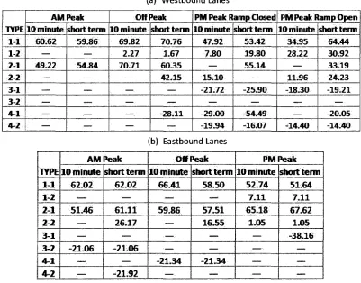
An average value was taken to determine typical speeds by shock wave type. Table 5-2 shows
the average shock wave values by type.
Table 5-2: Average Shock wave Speed by Type (Crash Cases) (a) Westbound Lanes
TYPE 1-1 1-2 2-1 2-2 3-1 3-2 4-1 4-2 AM Peak 10 minute 60.62 — 49.22 — — .<— — — short term 59.86 — 54.84 — — — .— — Off Peak 10 minute 69.82 2.27 70.71 — — — —. — short term 70.76 1.67 6035 42.15 — — -28.11 —
PM Peak Ramp Closed 10 minute 47.92 7,80 — 15.10 -21.72 .— -29.00 -19.94 short term 53.42 19.80 55.14 — -25.90 — -54.49 -16.07
PM Peak Ramp Open 10 minute 34.95 28.22 — 11:96 -18.30 — — -14.40 short term 64.44 30.92 33:19 24.23 -19.21 — -20.05 -14.40
(b) Eastbound Lanes
TYPE 1-1 1-2 2-1 2-2 3-1 3-2 4-1 4-2 AM Peak 10 minute 62.02 i — 51.46 — — -21.06 — short term 62.02 — 61.11 26.17 — -21.06 — -21.92 Off Peak 10 minute 66.41 —• 59.86 — .— — -21.34 — short term 58.50 •—••
5 7 3 1 16.55 — — -21.34 — PMPeak 10 minute 52.74 7.11 65.18 1.05 — —-— .— short term 51.64 7.11 67.62 1.05 -38.16 —• — —
For most cases, the average shock wave speeds are relatively similar. The only notable
exception is in the afternoon peak period for the ramp closed in the westbound lanes, which has
a value of -54.49 km/hr. As expected, the type 1-1 and type 2-1 shock waves produce the
highest shock wave values, because queue is either forming or dissipating solely in the
uncongested zone and a typical volume-density graph for shock waves shows a better trend in
the uncongested regime. Also, in real time, it is difficult to quantify speed, volume and
To identify the effect of shock wave on crash likelihood, shock waves were also estimated for
the normal traffic conditions when a crash did not occur. Shock waves were observed in the
same manner as the crash cases using the loop detector data obtained during normal traffic
conditions. These data are called "non-crash" data. The non-crash data were obtained from the
same detector station and at the same time period and weather conditions as the crash data but
on different weekdays when a crash did not occur. The purpose of this data extraction is to
control for the confounding effects of road geometry and weather on crash likelihood.
For the non-crash data, 43 cases (77%) in the 10-minute period and 46 cases (82%) in the short
term period of the eastbound lanes showed a type of shock wave, whereas for the westbound
lanes, 75 cases (66%) in the 10-minute period and 84 cases (74%) in the short term period
showed some type of shock wave. In every period, the non-crash data had more cases of shock
waves occurring than in the crash cases. It was found that the shock wave speeds differ for each
time period for crash and non-crash cases. The results are broken up again by shock wave type
as shown in Table 5-3.
Table 5-3: Shock waves by Shock wave Type (Non-Crash Cases) (a) Westbound Lanes
TYPE 1-1 1-2 2-1 2-2 3-1 3-2 4-1 4-2 NO TYPE TOTAL
A M Peak 10 minute 12 0 9 0 0 0 0 0 5 26 short term 1 1 0 1 1 0 0 0 1 0 3 26 Off Peak 10 minute 12 0 5 0 1 0 0 0 1 1 2 9 short term 13 0 4 0 2 0 1 0 9 2 9
PM Peak Ramp Closed 10 minute 9 2 4 1 2 0 1 0 9 28 short term 1 1 3 3 0 3 1 1 0 6 2 8