LIM, MIN YEOL. Improving Power and Performance Efficiency in Parallel and Distributed Com-puting Systems. (Under the direction of Dr. Vincent W. Freeh.)
For decades, high-performance computing systems have focused on increasing maximum
performance at any cost. A consequence of the devotion towards boosting performance significantly
increases power consumption. The most powerful supercomputers require up to 10 megawatts of
peak power – enough to sustain a city of 40,000. However, some of that power may be wasted with
little or no performance gain, because applications do not require peak performance all the time.
Therefore, improving power and performance efficiency becomes one of the primary concerns in
parallel and distributed computing. Our goal is to build a runtime system that can understand
power-performance tradeoffs and balance power consumption and power-performance penalty adaptively.
In this thesis, we make the following contributions. First, we develop a MPI runtime
sys-tem that can dynamically balance power and performance tradeoffs in MPI applications. Our syssys-tem
dynamically identifies power saving opportunities without prior knowledge about system behaviors
and then determines the best p-state to improve the power and performance efficiency. The system
is entirely transparent to MPI applications with no user intervention. Second, we develop a method
for determining minimum energy consumption in voltage and frequency scaling systems for a given
time delay. Our approach helps to better analyze the performance of a specific DVFS algorithm in
terms of balancing power and performance. Third, we develop a power prediction model that can
correlate power and performance data on a chip multiprocessor machine. Our model shows that the
power consumption can be estimated by hardware performance counters with reasonable accuracy
in various execution environments. Given the prediction model, one can make a runtime decision
of balancing power and performance tradeoffs on a chip-multiprocessor machine without delay for
actual power measurements. Last, we develop an algorithm to save power by dynamically
migrat-ing virtual machines and placmigrat-ing them onto fewer physical machines dependmigrat-ing on workloads. Our
scheme uses a two-level, adaptive buffering scheme which reserves processing capacity. It is
de-signed to adapt the buffer sizes to workloads in order to balance performance violations and energy
savings by reducing the amount of energy wasted on the buffers. Our simulation framework justifies
our study of the energy benefits and the performance effects of the algorithm along with studies of
by Min Yeol Lim
A dissertation submitted to the Graduate Faculty of North Carolina State University
in partial fullfillment of the requirements for the Degree of
Doctor of Philosophy
Computer Science
Raleigh, North Carolina
2009
APPROVED BY:
Dr. George N. Rouskas Dr. Gregory T. Byrd
Dr. Vincent W. Freeh Dr. Xiaosong Ma
Chair of Advisory Committee
DEDICATION
To my beautiful wife, Younghee Park,
my adorable son, Jaehyun,
and
BIOGRAPHY
Min Yeol Lim was born in Daegu, South Korea in 1974. He begun studying computing
engineer-ing at Kyungpook National University in Daegu, South Korea in 1993, and, after servengineer-ing Korea
military duty from 1995 to 1997, graduated with a Bachelor of Engineering degree in 2000. Then,
he continued his graduate study for a master degree at Korea Advanced Institute of Science and
Technology in Daejeon, South Korea. For two years, he focused on researching and developing a
load-balancing framework at Web application server farm, which is also the topic of his Master’s
thesis. After receiving the Master of Science degree in 2002, he worked at Supercomputing
Cen-ter of Korea Institute of Science and Technology Information where he conducted Grid computing
research. He began his doctorate study in the Department of Computer Science at North Carolina
State University in 2004. Since he joined the Operating System Research lab directed by Dr.
Vin-cent W. Freeh in 2005, he has focused his research on power/performance analysis and optimization
techniques for parallel and distributed computing systems. On August 14, 2009, he successfully
ACKNOWLEDGMENTS
I would like to thank all the people who helped me with this work. This dissertation could not have
been finished without their support.
First and foremost, I would like to appreciate Dr. Vincent W. Freeh who served as my
advisor as well as a mentor. It was an honor working with such a nice professor like Dr. Freeh. His
enthusiasm for the work kept me motivated and he always guided me to stay in the right direction
to my goal. He also supported me with kind advice and guidance on how to improve my spoken
and written skills. I would not have finished my degree on time without him. I truly appreciate his
tireless support at all levels.
I also would like to thank Dr. Xiaosong Ma, Dr. George Rouskas, Dr. Gregory Byrd,
and Dr. Robert Fowler for being members of my committee. They provided relevant, insightful
guidance to make good progress throughout my research. Their valuable comments helped me
focus on important issues and look at the big picture in my research.
I am grateful to many collaborators during my Ph.D. pursuit. Dr. David Lowenthal at
University of Arizona helped me take the first step to this dissertation. Through the collaboration
with him for my first paper, I learned how to conduct research in my area. Dr. Allan Porterfield was
a great mentor during my summer internship and academic year support at Renaissance Computing
Institute. I was able to make a significant progress and to broad my knowledge in my research by his
support. I also thank Daniel Bedard at Renaissance Computing Institute who developed PowerMon
device for his support in my research. I am grateful to Dr. Freeman Rawson at IBM who helped the
PADD research. I sincerely appreciate his invaluable advice and comments.
Finally, I would like to thank Tyler Bletsch during the years. He is a smart person who
has a lot of knowledge in computing systems. He was always willing to discuss my research and
gave great advice on this dissertation. He helped me understand and utilize all the systems in our
lab when starting my research from scratch.
I sincerely acknowledge the funding resources of my dissertation work: (1) NSF grants
(CCF-0234285 and CCF-0429643), (2) Dr. Vincent Freeh’s University Partnership award from
IBM, (3) PERI - Performance Engineering Research Center (PERC-3) DE-FC02-06ER25764, and
TABLE OF CONTENTS
LIST OF TABLES . . . vii
LIST OF FIGURES . . . . ix
1 Introduction . . . . 1
1.1 Power and performance tradeoffs . . . 2
1.2 Accomplishments . . . 3
1.3 Contributions . . . 5
2 Background . . . . 6
2.1 Energy savings in server systems . . . 6
2.2 Energy savings in HPC systems . . . 7
2.3 Energy savings in server farms . . . 9
3 Adaptive, Transparent CPU Scaling Algorithms in MPI Communications . . . 12
3.1 Motivation . . . 13
3.2 Design and implementation . . . 18
3.2.1 The training component . . . 18
3.2.2 The shifting component . . . 22
3.3 Results . . . 24
3.3.1 Overall results . . . 28
3.3.2 Detailed analysis . . . 32
3.4 Summary . . . 40
4 Determining the Minimum Energy Consumption . . . 41
4.1 Approach . . . 42
4.1.1 Modeling . . . 43
4.1.2 Scheduling algorithm . . . 44
4.2 Implementation . . . 46
4.2.1 Time and energy data collection . . . 46
4.2.2 Power measurements . . . 48
4.2.3 Finding regions . . . 49
4.3 Results . . . 50
4.3.1 Detailed analysis . . . 51
4.3.2 Discussion . . . 54
5 Fine-grained and Accurate Power Measurements . . . 56
5.1 Design . . . 58
5.2 Evaluation . . . 60
5.2.1 Access latency and accuracy . . . 60
5.2.2 Fine-grained power measurement . . . 62
5.2.3 Power monitoring overhead . . . 66
5.2.4 Power supply efficiency . . . 67
5.3 Summary . . . 69
6 Power Prediction on Multi-core system via Performance Counters . . . 70
6.1 Approach . . . 71
6.1.1 Measuring power and performance . . . 71
6.1.2 Profiling power and performance . . . 71
6.1.3 Selection of performance counters . . . 72
6.1.4 Applying multivariate linear regression . . . 72
6.2 Evaluation . . . 74
6.3 Summary . . . 80
7 PADD: Power Aware Domain Distribution . . . 81
7.1 Model . . . 83
7.1.1 Machine State and virtualization . . . 83
7.1.2 Model description . . . 84
7.2 Implementation . . . 86
7.2.1 Buffering . . . 87
7.2.2 Time cost of transitions . . . 88
7.2.3 Additional parameters . . . 89
7.2.4 Algorithm . . . 90
7.3 Evaluation . . . 91
7.3.1 Workload generation . . . 91
7.3.2 System configuration . . . 92
7.3.3 Analysis . . . 93
7.4 Summary . . . 98
8 Concluding remarks . . . 100
8.1 A runtime power-performance directed adaptation . . . 100
8.2 Dynamic power efficiency adaptation on multi-core architecture . . . 101
8.3 Conclusion . . . 103
LIST OF TABLES
Table 3.1 Analysis of MPI call length and interval between MPI calls per benchmark.
Bench-marks are sorted by 75th percentile in ascending order. . . 17
Table 3.2 P-state transition cost (microseconds) for a AMD Athlon-64 3000+ Processor [1]. The frequency in a row indicates a starting p-state and the frequency in a column is a target p-state. . . 24
Table 3.3 Benchmark attributes. Region information from composite with τ = 20 ms and λ= 20ms. . . 25
Table 3.4 Overall performance of benchmark programs. Where appropriate, the value relative to the base case is also reported. . . 29
Table 3.5 Performance comparison between single p-state and automatic multiple p-state selec-tion. . . 33
Table 4.1 Analysis per region in LU benchmark . . . 44
Table 4.2 The workload analysis of finding the best schedule . . . 51
Table 4.3 Estimation verification . . . 52
Table 5.1 Comparison of PowerMon and Power Egg access latencies. Power Egg requires at least 480 ms between requests. . . 60
Table 5.2 Measured hard disk power consumption . . . 65
Table 5.4 Power supply efficiency by CPU loads on a quad-core Intel Nehalem machine . . . 68
Table 6.1 Correlation of selected performance counters with internal power consumption . . . 75
Table 6.2 Three selected performance counter groups and their coefficients of determination of multivariate regression . . . 75
Table 7.1 Parameters defined for PADD and its power and performance model . . . 84
LIST OF FIGURES
Figure 1.1 Effect of DVFS in energy consumption . . . 3
Figure 3.1 Micro-benchmarks showing time and energy performance of MPI calls with CPU scaling. . . 14
Figure 3.2 Micro-benchmarks showing time and energy performance of MPI calls with CPU scaling. . . 15
Figure 3.3 Cumulative distribution functions (CDF) of the duration of and interval between MPI calls for every MPI call for twelve benchmark programs we evaluate in this chapter. 16
Figure 3.4 This is an example trace of an MPI program. The line shows the type of code executed over time. There are 10 MPI calls, and calls 1–3 and 5–8 make up communication regions because they are close enough. Call 9 is considered a region because it is long enough. Even though they are MPI calls, calls 4 and 10 are not in a communication region because they are neither close enough nor long enough. . . 19
Figure 3.5 The mapping of OPS to P-state for a communication region. . . 21
Figure 3.6 State diagram for composite algorithm. . . 23
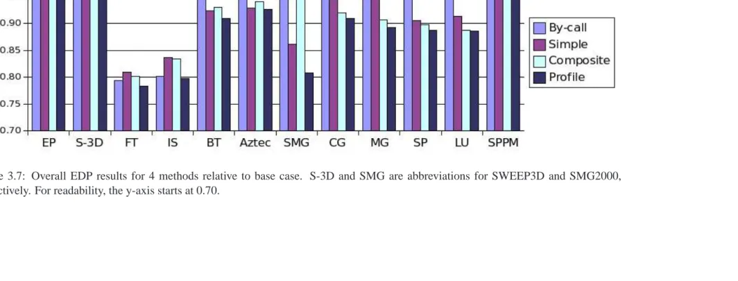
Figure 3.7 Overall EDP results for 4 methods relative to base case. S-3D and SMG are ab-breviations for SWEEP3D and SMG2000, respectively. For readability, the y-axis starts at 0.70. . . 27
Figure 3.8 Comparison of single and multiple p-state transition. S-3D and SMG are abbre-viations for SWEEP3D and SMG2000, respectively. For readability, the y-axis starts at 0.70. . . 31
Figure 3.9 These are p-state transition examples by different MPI call patterns. FN and FP mean false negative and false positive, respectively. . . 35
Figure 3.10 Breakdown of execution time for adaptive region-finding algorithms withτ = 20 ms andλ= 20ms. . . 36
Figure 3.12 Evaluatingτ in composite. Show fraction of time mispredicted and number of re-gions (right-hand y-axis) as a function ofτ. For readability, right-hand y-axis has different
scale for CG and SP. (Continuation of Figure 3.11.) . . . 39
Figure 4.1 Execution time vs. energy consumption from single p-state execution . . . 47
Figure 4.2 Execution time vs. energy consumption from single p-state execution . . . 48
Figure 4.3 Execution time vs. energy consumption per region . . . 50
Figure 4.4 Minimum energy over time . . . 53
Figure 5.1 PowerMon prototype board . . . 58
Figure 5.2 A reading from different sensors . . . 59
Figure 5.3 Accuracy comparison of internal and external power meters. . . 61
Figure 5.4 PowerMon and Power Egg measurements with different active thread/core counts . 63 Figure 5.5 PowerMon and Power Egg measurements running Iperf benchmark. . . 64
Figure 5.6 PowerMon and Power Egg measurements with different PCI cards installed. . . 65
Figure 5.7 PowerMon and Power Egg power measurements with/without a hard drive. . . 66
Figure 5.8 Power consumption over different monitoring intervals. . . 67
Figure 6.1 Distribution of prediction errors . . . 76
Figure 6.2 Power Prediction Accuracy for NPB benchmark . . . 77
Figure 6.3 Power Prediction Accuracy for SPECOMP benchmark . . . 78
Figure 7.1 Node and Domain state diagrams. Each edge indicates the transition time delay. . . 83
Figure 7.2 Each node has its own Local Buffer. The Global Buffer is a pool of additional capacity spread across the active nodes. . . 87
Figure 7.4 Average power consumption and CPU utilizations for 11 different load levels. The power consumption is obtained from the SPECpower ssj2008 benchmark. While running it, the CPU utilizations are measured in the same machine. . . 91
Figure 7.5 The overall comparison of the representative cases. (Util=14.5%, MW=60, AP=60, VS=1, MD=30) . . . 93
Figure 7.6 The comparison of the adaptive GB/LB with different workload intensity. (MW=60, AP=60, VS=1, MD=30) . . . 93
Figure 7.7 The comparison of adaptive buffering and fixed buffering. (Util=14.5%, MW=60, AP=60, VS=1, MD=30) . . . 94
Figure 7.8 The comparison of domain migration and node transition cost. (Util=14.5%, MW=60, AP=60, VS=1, MD=30) . . . 95
Chapter 1
Introduction
In the past decades, the “performance only” paradigm in high performance parallel and
distributed computing systems tends to increase performance at all costs. The attention given to
increasing computing performance has resulted in excessive power usage in two ways: drawing
more power by CPU itself and dissipating more heat generated by CPU. As an example of the
problem that is faced, several years ago it was observed that on their current trend, the power density
of a microprocessor will reach that of a nuclear reactor by the year 2010 [2]. According to Eric
Schmidt, CEO of Google, what matters most to Google is not speed but low power, because data
centers can consume as much electricity as a small city. The 10 most powerful supercomputers on
the TOP500 List (www.top500.org) each require up to 10 megawatts of peak power – enough to
sustain a city of 40,000 [3]. As a result, power-aware computing has been recognized as one of
critical research issues in parallel and distributed computing systems.
Our goal is a system that can understand power-performance tradeoffs and balance power
consumption and performance. The system collects relevant data at runtime and evaluate the
trade-offs using empirical observations. Then, it dynamically and efficiently changes the execution
en-vironment of running an application in order to improve power and performance efficiency. This
thesis shows our accomplishments to achieve our goal.
In this work, we develop and evaluate several systems that can understand different power
and performance tradeoffs by characterizing application behaviors and take advantage of these
char-acteristics. Our systems figure out the tradeoffs at runtime and make the best power saving decision
on the fly among available power saving techniques. We show that the adaptive methods achieve
1.1
Power and performance tradeoffs
Unfortunately, the “last drop” of performance tends to be the most expensive. One reason
is power consumption, because dynamic power is proportional to the product of the frequency and
the square of the voltage. A simple model of dynamic power consumption (P) of a CPU
imple-mented in CMOS technology is approximated as follows:
P ≈A C V2 f + L
where C is total capacitance, A is CPU activity, f is frequency, V2
is the square of voltage, and
L is leakage by static power. In recent computing systems, the static power becomes a significant
component of total power dissipation [4]. It can be comparable to dynamic (switching) power in
future technologies. Reducing the static power, however, is a hardware design issue.
Energy consumption (in Joules) is measured by integrating the production of
instanta-neous power (P(t)) by time;
E =
Z t2
t1
P(t)dt
To dynamically balance the concerns of power and performance, new architectures have aggressive
power controls. Because architectural advances for raw performance improvement are accompanied
with more power usage, several power-aware computing techniques have been introduced to control
both power and performance dynamically. For example, many microprocessors allow frequency
and voltage scaling on the fly, which allows the application or operating system to provide dynamic
voltage and frequency scaling (DVFS). DVFS is a popular and effective technique, performed in
adjusting a power-performance tradeoff because CPU is the major power consumer in a single
node, consuming 35-50% of the nodes’ total power [5]. We denote each possible combination
of voltage and frequency a processor state, or p-state.1 While changing p-states has broad utility, including extending battery life in small devices, the primary benefit of DVFS occurs when the
p-state is reduced in code regions where the CPU is not on the critical path. In such a case, power
consumption will be reduced with little or no decrease in end-user performance.
Figure 1.1 shows the energy-time (or, equivalently, power-performance) tradeoff
graphi-cally. The rectangular area in Figure 1.1(a) shows the energy consumption at the highest frequency.
1
(a) Before Scaling
! " #" #$ % &'(&) * !+ #+ ,-. -/01 2 34 1 56!+7#+
(b) After Scaling
Figure 1.1: Effect of DVFS in energy consumption
On the other hand, Figure 1.1(b) shows the change of energy consumption to a lower frequency
after p-state transition. Once we scale the CPU voltage and frequency, a cubic drop in power usage
occurs. However, the performance decrease is at most linear with frequency reduction, which
(usu-ally) increases overall execution time. So, the overall energy savings can be realized only if cost is
less than benefit. In high performance computing, Energy-Delay Product (EDP) is commonly used
to evaluate the power-performance tradeoff. This metric is more biased toward execution time than
the Energy metric. In this research, we use different metrics depending on the characteristics of
applications.
1.2
Accomplishments
Our goal is to balance power savings and performance penalty in parallel or distributed
applications by exploiting various power saving techniques. This dissertation consists of five related
projects that we accomplished. Each project plays a vital role as a steppingstone to the goal.
Chap-ter 3 describes a MPI runtime system that dynamically reduces CPU frequency and voltage during
communication phases in MPI programs. It dynamically identifies such phases and, without
pro-filing or training, selects the CPU frequency in order to balance power-performance tradeoffs (i.e.,
energy-delay product). All analysis and subsequent frequency and voltage scaling is performed
via MPI profiling interface and so is entirely transparent to the application. This means that the
without modification. Results show that the median reduction in energy-delay product for twelve
benchmarks is 8%, the median energy reduction is 11%, and the median increase in execution time
increase is only 2%.
In Chapter 4, we determine minimum energy consumption in voltage and frequency
scal-ing systems for a given time delay. As we mentioned earlier, The benefit of DVFS varies by
work-load characteristics in code regions. Therefore, it is difficult to evaluate the effectiveness of a DVFS
scaling algorithm. Our work establishes the optimal baseline of DVFS scheduling for any
applica-tion. Given the baseline, one can better evaluate a specific DVFS technique. We assume we have
a set of discrete places where scaling can occur. A brute-force solution is intractable even for a
moderately sized set (although all programs presented can be solved with the brute-force approach).
Our approach efficiently chooses the exact optimal schedule satisfying the given time constraint by
estimation. We evaluate our time and energy estimates in NPB serial benchmark suite. The results
show that the running time of the algorithm can be reduced significantly with our algorithm. Our
time and energy estimations from the optimal schedule have high accuracy, within 1.48% of actual.
Chapter 5 describes an internal power meter that provides accurate, fine-grained
measure-ments. The above projects use the entire system power consumption to quantify the effectiveness.
However, the power consumed by each component within a system actually varies during program
execution. External power measurements do not provide information about how the individual
com-ponents utilize power. The fine-grained monitoring of the prototype is evaluated and compared with
the accuracy and access latency of an external power meter. The results show that we can measure
the power consumption more accurately and more frequently (about 50 measurements per second)
with low power monitoring overhead (about 0.44 W). When combined with an external power meter,
we can also derive the power supply efficiency and the hard disk power consumption.
Chapter 6 describe how to estimate the power consumption with performance data
ob-served in a system. For this prediction model, we profile the power and performance data when
running multi-threaded applications on multi-core architecture and then establish a power
predic-tion model using a regression method. We evaluate and analyze the accuracy of this predicpredic-tion
model.
In Chapter 7, we develop a power-aware domain placement solution in virtualized system
environments. This technique saves power by dynamically migrating virtual machines and packing
them onto fewer physical machines when possible. We perform a simulation study on this
outperforms in terms of energy savings.
In Chapter 8, we conclude our research by summarizing our accomplishments. Also, we
present future research directions in our research area. In addition to the previous accomplishments,
we still strive for improving runtime adaptation of power-performance in parallel applications. The
adaptation will achieved through continuous power and performance monitoring by primarily
ex-ploiting DVFS. We also plan to explore various adaptation technique, such as the number of active
threads in OpenMP applications if useful.
1.3
Contributions
In this work, we make the following contributions. First, we develop a MPI runtime
system that can dynamically balance power and performance tradeoffs in MPI applications by
min-imizing energy-delay product. Our system dynamically identifies power saving opportunities
with-out profiling or training and then determines the best p-state to improve the power and performance
efficiency Our system is entirely transparent to MPI applications because it works within MPI
li-brary.
Second, we develop a method for determining minimum energy consumption in voltage
and frequency scaling systems for a given time delay. Our method efficiently chooses the exact
opti-mal schedule satisfying a given time constraint by estimation. Our approach helps to better analyze
the performance of a specific DVFS algorithm in terms of balancing power and performance.
Third, we develop a power estimation model that can correlate power and performance
data on a chip multiprocessor machine. According our evaluations, the prediction model is
reason-ably accurate to predict power consumption only with performance data in various execution
con-figurations. While running an application, one can make a fast decision of power and performance
adaptation by using performance data, because there is no delay for actual power measurements.
Last, we develop an algorithm to save power by dynamically migrating virtual machines
and placing them onto fewer physical machines depending on their performance needs. Our scheme
uses a two-level, adaptive buffering scheme which reserves processing capacity. It is designed to
absorb workload surges to avoid significant performance violations, while reducing the amount of
energy wasted on the buffers. We also develop a simulation framework for our study of the energy
benefits and the performance effects of our algorithm along with studies of its sensitivity to various
Chapter 2
Background
Power and energy savings have been one of main issues in many computing research area.
In this chapter, we describe the related work by making two parts in order to describe diverse ways
of previous research. First, we summarize prior work for power savings in mobile / server systems.
Then, the power savings research focusing on HPC systems are presented.
2.1
Energy savings in server systems
Originally, much work in energy savings has been aimed at the systems that operate on
energy-constrained devices, such as mobile systems. The goal is to develop an efficient energy
savings algorithm either through dynamic voltage and frequency scaling (DVFS) [6, 7, 8] or through
disk / network control [9, 10] while, at the same time, satisfying system requirements. In this
dissertation, we focus on energy savings in parallel and distributed server systems, instead of mobile
systems. This research is complementary to ours and provides a worthwhile guidance.
Several projects have also examined energy savings in server systems. Energy savings
has become one of the biggest concerns, especially those sites which have server farms, such as
hosting centers managing sufficiently large numbers of machines. In these sites, energy
manage-ment may become an issue; see [11, 12, 13] for examples of this using commercial workloads and
web servers. Such work shows that power and energy management are critical for commercial
workloads, especially web servers [14]. Additional approaches have been taken to include DVFS
and request batching [15]. The work in [16] applies real-time techniques to web servers in order
evaluates the impacts of DVFS in terms of quality of service as well as power savings. One is to
propose a DVFS algorithm meeting the end-to-end delay constraint in web servers [17]. The other
[18] shows, given tolerable response time, the possible power savings in a Web server testbed. The
paper [19] proposes a framework for improving the aggregate throughput by controlling the power
allocation in multiple system under a certain power limitation. The papers [20, 21] show that
effi-cient algorithms for server load balancing can be one promising solution. On the other hand, various
methods have been proposed to achieve energy savings by applying power-scalable components to
either CPU or disk, which are two major power consumers [22]. Most work focuses on leveraging
power (energy) performance tradeoffs under given conditions such as maximum bound of power
consumption and tolerable performance.
In server farms, disk energy consumption is also significant; several groups have studied
reducing disk energy by reducing disk access speed or by varying its energy level (e.g., [23, 24, 25]).
The approach in the paper [26] infers disk access patterns of application with program counters,
which can allow avoidance of unnecessary disk energy consumption. In our work, we do not
con-sider disk energy savings as it is generally less than CPU energy, especially if scientific programs
operate primarily in core.
Our work differs from prior research in that it focuses on HPC systems which execute
scientific applications specifically, rather than mobile devices or commercial servers. Commercial
workloads vary over time. Therefore, energy management is often performed by a conservative
method which is used according to the service load. On the other hand, HPC applications often
have regular patterns and they are more predictable than commercial workloads. Our work aims
at efficiently applying DVFS with imposed time delay in a fine-grained way to maximize energy
savings effect. Thus, the prior research in disk energy management is complementary to ours.
2.2
Energy savings in HPC systems
The most relevant related work to this dissertation is in high-performance, power-aware
computing. For decades, performance improvement for both systems and applications has been the
only major consideration in HPC research areas. Consequently, it resulted in the advent of large
scale power consuming clusters, which causes substantial energy cost. Hence, much research for
power awareness in HPC community has been introduced recently.
deploying digital multi meters. The profiling framework isolates 10 power points including CPU,
memory, disk, and network and profiles power changes while running some benchmarks. Although
its profiling approach is similar with ours, the approach is not flexible in that the monitoring
frame-work is dedicated to its testing cluster machines. The paper [28] introduces a dynamic compilation
technique of HPC applications to reduce power consumption. This work focuses only on I/O
op-timization in order to save both time and energy. Ge et al. [29] uses a variety of different DVFS
scheduling strategies (for example, both with and without application-specific knowledge) to save
energy without significantly increasing execution time. Follow-on work saved energy while limiting
the execution time overhead to a user-specified amount [30]. A similar run-time effort is described
by Hsu and Feng [31]. The prior work at NC State is fourfold: an evaluation-based study that
fo-cused on exploring the energy/time tradeoff in the NAS suite [32], development of an algorithm
for switching p-states dynamically between phases [33], leveraging load imbalance by inter-node
bottleneck to save energy [34], and minimizing execution time subject to a cluster energy constraint
[35]. Another recent work [5] exploited inter-node slack time to reduce power consumption. The
algorithm automatically identifies idle time at the end of each iteration and then steers the p-state
for energy savings. This is an effective approach, especially in a load unbalanced job execution,
such as N-Body simulation.
The above approaches strive to save energy for a broad class of scientific applications.
Another approach is to save energy in an application-specific way; work by Chen et al. [36] used
this approach dedicated to a parallel sparse matrix application, and Hsu and Kremer [37] leverage
the memory bottleneck of HPC applications.
Recently, Curtis-Maury et al. [38] developed an adaptive concurrency control framework
in OpenMP applications. This utilizes multiple thread-to-core mappings in multi-core
architec-ture. This approach establishes a performance model for accurate power-performance prediction.
Their following work [39] expands the approach by integrating DVFS. They achieved good
power-performance adaptation on multi-core architecture. However, there exist several limitations. First,
the approach only can be applied for OpenMP based applications. Second, the adaptation needs
priori information that is used to train a system for accuracy. Different tuning is required on a
dif-ferent machine. Third, they do not provide in-depth analysis regarding their power-performance
adaptation they achieved.
In addition to designing energy saving algorithms, determining the maximum bound of
achieve-ment of energy savings itself does not explain the comparable value of the algorithms unless the
possible savings at maximum is known. This research can establish the potential benefit of DVFS
for a given application.
There are also a few high-performance computing clusters designed with energy in mind.
One is BlueGene/L [42], which uses a “system on a chip” to reduce energy. While each node
consumes little energy and has low performance, high performance is achieved by using up to
128,000 processors. An earlier energy-aware machine, Green Destiny [43], uses low-power
Trans-meta nodes.
Our work attempts to infer regions based on recognizing repeated execution. Others have
had the same goal and carried it out using the program counter. Gniady and Hu used this technique
to determine when to power down disks [44], along with buffer caching pattern classification [45]
and kernel prefetching [46]. In addition, dynamic techniques have been used to find program phases
[47, 48, 49], which is tangentially related to our work. We divide programs into one or more
com-munication phases. There has been a large body of work in phase partitioning. Static techniques,
such as [50, 51], appeared in the literature first.
2.3
Energy savings in server farms
Much research has been conducted on dynamic mapping of domains to physical machines.
In some work, performance is the primary concern without power analysis. The work by Steinder, et
al. [52], is both implementation and a simulation. In her work, there is a workload flow controller
that manages the workloads being run and helps drive the application placement controller. In our
work, there is no such workload controller: the workloads are run in the individual domains without
any centralized control over them. The study by Bobroff, et al. [53], is a predictive placement
scheme based on time series analysis. In contrast, our work is reactive, observing load and reacting
appropriately.
The problem of saving power in a throughput-computing environment has also been
stud-ied previously. Most work centers on fluid workloads, i.e., workloads consisting of many short-lived
independent requests that can be served by homogeneous software running on multiple physical
ma-chines and which have a centralized workload distributor that routes the requests to the mama-chines
which process them. Elnozahy, et al. [54] simulate the effects of dynamic voltage scaling coupled
two well-known production web traces and find that VOVO alone saves up to 42 % while the
ad-dition of voltage scaling saves an adad-ditional 18 %. Similarly, Chase, et al. [55] use an artificial
resource economy to save energy by balancing the cost of resources against the benefit realized by
employing them. This is also simulation-based work and focuses on satisfying the demand presented
by web traffic traces. Both techniques save power by turning some nodes off and using a central
workload distributor to route new requests to other nodes. The Power-Aware Request Distribution
(PARD) system addresses data center power by using the individual request as the fundamental unit
of work [56]. The system directs requests to a pool of compute resources which can be powered on
or off depending on anticipated load. Because requests are independent and servers are stateless,
powering down a server is simply a matter of removing it from the load balancer, waiting for
pend-ing requests to finish, and turnpend-ing it off. In this environment, there is nothpend-ing to migrate or back
up when shutting down a node, which leads to a very fine-grained power management: the system
runs only the machines needed to satisfy the current demand. However, the PARD approach is only
applicable to workloads similar to web-serving, and many workloads cannot be modeled in this
manner. For example, processes may need to maintain state, or there may be multiple indivisible
processes that each handle a separate incoming demand.
Recently, Nathuji and Schwan [57] proposed a framework to determine the power-performance
tradeoffs of virtual machines and to efficiently manage physical machines within given power
bud-gets. This work focuses on achieving good performance under a power cap, whereas our work seeks
to satisfy an SLA while minimizing energy consumption. Verma, et al. [58, 59] designed and
eval-uated several domain placement algorithms on top of their existing platforms. Like our approach,
they examined the tradeoff between power consumption and migration cost of running domains
when determining their placement in virtualized systems. Although the problem they are
address-ing is similar, our contribution is distaddress-inguished in two ways. First, because our work is a simulation
study, we can define and explore numerous configurable parameters that vary by hardware and
soft-ware characteristics and evaluate their effects in theoretical environments, including very large scale
computing systems. Second, we propose a two-level buffering scheme where the buffering sizes are
adapted by given SLA requirements. Our algorithm finds power efficient placement of domains
while minimizing the SLA violation.
There has been a significant amount of research into understanding and predicting
work-load patterns. Bradley, et al. [60] proposed two power management algorithms using short-term and
enough available resources proactively by exploiting these patterns. More recently, Chen, et al. [61]
studied incoming traffic patterns and used them to predict the amount of resources needed to
pro-cess the load. Such prior work focuses on improving predictions of workloads and applying the
information to power aware server provisioning. In contrast, PADD simply reacts to the work being
processed or being generated within the computing environment. In addition, these studies assume
that one server is dedicated to a service. Since the servers are not shared by different services, there
is no domain migration between running servers. These approaches are complementary to our work
because combining prediction with reaction to the workload can lead to better placement decisions,
achieving more power savings with less performance impact.
In contrast to coarse-grained domain packing, CPU packing and node packing techniques
[62, 63, 64] are available to the operating system as a fine-grained packing. This allows the packing
of jobs onto a subset of the available processors and power down the rest.
There is a large body of work on Dynamic Voltage and Frequency Scaling (DVFS) to
save energy [65, 66]. The work [67] proposes a online power management approach on a virtual
machines supporting isolation between them and honoring the power management requests of the
individual virtual machines. Using DVFS allows us to improve further the power efficiency of the
running systems in the environment by reducing voltage and frequency when a server’s processors
are not a bottleneck. Since our work aims at domain distribution in virtualized server environments,
any local DVFS algorithm in a system can be combined with our approach to get additional power
Chapter 3
Adaptive, Transparent CPU Scaling
Algorithms in MPI Communications
In this chapter, we present a transparent, adaptive system that reduces the p-state in
com-munication phases. While changing p-states has broad utility, including extending battery life in
small devices, the primary benefit for HPC occurs when the p-state is reduced in regions where the
CPU is not on the critical path. In such a case, power consumption will be reduced with little or no
reduction in end-user performance. Previously, p-state reduction has been studied in code regions
where the bottleneck is in the memory system [68, 31, 29, 32, 33] or due to load imbalance between
nodes [34]. In our approach, the communication phase is defined as a code region of applications
calling Message Passing Interface (MPI).
Our system is built as two integrated components: training the system and making the
actual shifting. We first designed several training algorithms that demarcate communication regions.
In addition, we use a simple metric — operations per unit time — to determine the proper p-state
for each region. To do so, it monitors MPI calls to determine communication regions on the fly.
We then designed the shifting component, which includes the mechanics of reducing the p-state at
the start of a region and increasing it at the end. Once regions are demarcated, our system uses
performance counters to choose the appropriate p-state for each communication region; that is, at
the beginning of the region it reduces the p-state to the region-specific target, and at the end of the
region it increases the p-state back to its original setting.
Because our system is built strictly with code executed within the PMPI runtime layer,
there is no user involvement whatsoever. Thus, the large base of current MPI programs can
uti-lize our technique with both no source code change and no recompilation of the MPI runtime
li-brary. While we aim our system at communication-intensive codes, the performance degradation
for computation-intensive programs is negligible.
The difference between all the research presented in Section 2.2 and this chapter is the
type of bottleneck we are attacking. Specifically, researchers have attacked both the memory
bottle-neck, where energy can be saved because the CPU is waiting for data from the memory system, and
the node bottleneck, where energy can be saved because the CPU is waiting for data from another
node. Here, we address the communication bottleneck, where energy can be saved because MPI
communication operations are not CPU intensive. This is the first work we know of to address the
communication bottleneck.
Results on the NAS benchmark suite and the ASCI Purple benchmark suite show that
we achieve up to a 19.9% reduction in energy-delay product (EDP) compared to an energy-unaware
scheme where nodes run as fast as possible. Furthermore, across the entire NAS suite, our algorithm
that reduces the p-state in each communication region saved an median of 8% in EDP and 11% in
energy. This was a significant improvement compared to simply reducing the p-state for each MPI
communication call. Also, importantly, this reduction in EDP did not come at a large increase in
execution time; the median increase across all benchmarks was 1.9%, and the worst case was only
5.8%.
The rest of the chapter is organized as follows. In Section 3.1, we provide motivation
for reducing the p-state during communication regions. Then, Section 3.2 discusses our
imple-mentation, and Section 3.3 discusses the measured results on our power-scalable cluster. Finally,
Section 3.4 summarizes and describes future work.
3.1
Motivation
To be effective, reducing the p-state of the CPU should result in a large energy savings
but a small time delay. We implemented a microbenchmark that repeatedly calls the same MPI
operation with a fixed message size. We executed this microbenchmark on 2 nodes for about 50
seconds using many common MPI operations using both small and large messages. Figures 3.1
0.4 0.6 0.8 1 1.2 800 1200 1600 2000 Frequency (MHz) Size = 2 KB
time energy 0.4 0.6 0.8 1 1.2 800 1200 1600 2000 Frequency (MHz) Size = 40 KB
time energy
(a)MPI Recv
0.4 0.6 0.8 1 1.2 800 1200 1600 2000 Frequency (MHz) Size = 2 KB
time energy 0.4 0.6 0.8 1 1.2 800 1200 1600 2000 Frequency (MHz) Size = 40 KB
time energy
(b)MPI Send
0.4 0.6 0.8 1 1.2 800 1200 1600 2000 Frequency (MHz) Size = 2 KB
time energy 0.4 0.6 0.8 1 1.2 800 1200 1600 2000 Frequency (MHz) Size = 40 KB
time energy
(c)MPI Alltoall
Figure 3.1: Micro-benchmarks showing time and energy performance of MPI calls with CPU scaling.
represents time and energy values relative to the fastest frequency (or p-state). For all the MPI
operations (including those not shown), the p-state with frequency 1000 MHz provides an excellent
tradeoff between time and energy: at least 20% energy is saved with a time increase of at most 2.6%.
0.4 0.6 0.8 1 1.2 800 1200 1600 2000 Frequency (MHz) Size = 2 KB
time energy 0.4 0.6 0.8 1 1.2 800 1200 1600 2000 Frequency (MHz) Size = 40 KB
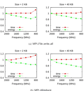
time energy
(a)MPI File write all
0.4 0.6 0.8 1 1.2 800 1200 1600 2000 Frequency (MHz) Size = 2 KB
time energy 0.4 0.6 0.8 1 1.2 800 1200 1600 2000 Frequency (MHz) Size = 40 KB
time energy
(b)MPI Allreduce
Figure 3.2: Micro-benchmarks showing time and energy performance of MPI calls with CPU scaling.
On the other hand, there often is a large time penalty using the slowest frequency (800 MHz) for
sending small messages, up to 17%. For large messages, 800 MHz has a time increase as large as
5%. Overall, these data show that MPI calls provide an excellent opportunity to save energy with
little or no time penalty.
However, in practice, an MPI operation may be too short to make reducing the p-state
before and increasing the p-state after every call effective. The problem exists because p-state
tran-sitions are not instantaneous. Therefore, a short MPI operation does not have sufficient benefit
to overcome the transition cost. Figure 3.3(a) shows a cumulative distribution function (CDF) of
elapsed times of all MPI calls in all 12 benchmarks evaluated in this chapter (the entire NAS
bench-mark suite and four ASCI Purple benchbench-marks). These data are obtained from executions on 8 or 9
nodes on AMD Athlon-64 cluster connected by a 100Mbps network (see Section 3.3 for a complete
0 0.1 0.2 0.3 0.4 0.5 0.6 0.7 0.8 0.9 1
0 5 10 15 20
Fraction of calls
Call length (ms)
(a) CDF of MPI call length
0 0.1 0.2 0.3 0.4 0.5 0.6 0.7 0.8 0.9 1
0 5 10 15 20
Fraction of calls
Call length (ms)
(b) CDF of inter MPI call interval
Figure 3.3: Cumulative distribution functions (CDF) of the duration of and interval between MPI calls for every MPI call for twelve benchmark programs we evaluate in this chapter.
so a communication-intensive benchmark has greater influence on this figure than a benchmark with
few messages.) This figure shows that over 97% of MPI calls take less than 10 ms and 78% take
less than 1 ms.
Considering that changing the p-state averages 1200 microseconds and can take up to
5600 microseconds (See Section 3.2.2 for details), time (and energy) increases when one reduces
the p-state for each MPI operation and only for the duration of the operation. Figure 3.3(b) plots
the CDF for the interval between MPI calls from the same experiments above. It shows that
three-fourths of all intervals are less than 1 millisecond, indicating that MPI calls are clustered in time.
Therefore, we can group “adjacent” MPI calls together as a region, avoiding frequent p-state
transi-tions. Shifting only at region boundaries amortizes the overhead of p-state transitions, but executes
the non-MPI code between calls in a reduced p-state, which may not be ideal.
The data presented in Figure 3.3 is an aggregate of all benchmarks. However, benchmarks
have different communication patterns. Table 3.1(a) shows MPI call length per benchmark. (EP,
which has only 5 MPI calls, is not shown.) The table shows the first, second, and third quartiles,
sorted by the third quartile (column 3). The table shows that for 7 of 11 benchmarks, more than
three-fourths of their MPI operations take less than 1 millisecond. Table 3.1(b) shows the detailed
analysis of the inter-MPI intervals per benchmark. These data are again sorted by the third quartile;
however, the order is different. It shows that for 5 benchmarks over three-fourths of the intervals
take less than 1 millisecond. Also, the median interval is less than 1 millisecond for 8 benchmarks.
Table 3.1: Analysis of MPI call length and interval between MPI calls per benchmark. Benchmarks are sorted by 75th percentile in ascending order.
Benchmark 25% 50% 75%
Aztec 0.01 0.01 0.03
SMG2000 0.01 0.01 0.03
MG 0.04 0.07 0.11
LU 0.04 0.08 0.14
SPPM 0.01 0.06 0.39
CG 0.02 0.05 0.52
SWEEP3D 0.15 0.30 0.56
BT 6.52 6.71 6.97
SP 0.02 0.10 17.9
IS 0.47 41.8 10124
FT 1.47 1698 38541
(a) Analysis of MPI call length (ms).
Benchmark 25% 50% 75%
Aztec 0.01 0.02 0.03
SMG2000 0.01 0.02 0.03
BT 0.03 0.03 0.03
CG 0.01 0.03 0.48
MG 0.03 0.28 0.91
LU 0.07 2.37 2.66
SPPM 0.01 0.11 10.3
SWEEP3D 0.13 0.20 33.2
SP 0.03 6.21 34.2
IS 0.03 0.06 624
FT 2403 2937 3743
(b) Analysis of time interval (ms) between MPI calls.
MPI operations, so there is no need to amortize the shifting overhead over multiple operations. The
tables foretell a problem in SWEEP3D, which has many short operations but a rather long
third-quartile interval.
Because there is a cost to p-state shifting, it is necessary to avoid shifting too frequently.
The data in these table show that the vast majority of MPI operations are too short to justify p-state
shifting. However, the data also show that operations are clustered very close together. This presents
an opportunity to be amortize the overhead of shifting across multiple MPI operations. Because it
is unlikely that there is significant computation in the short code sections between MPI, the penalty
for reducing the p-state in non-communication code is not expected to be great. Therefore, this
project considers closely clustered MPI operation and the code between them to be communication
regions, which are candidates for executing in a reduced p-state and saving energy.
Finally, our solution only considers shifting at MPI operations. However, there are other
places shifting can be done. For example, one could shift at program (or computational) phase
boundaries or even at arbitrary intervals. We rejected the latter because such shifting is not
context-sensitive, meaning that we could not learn from previous iterations. The former is context-context-sensitive,
and with elaborate phase analysis it will likely find excellent shifting locations. However, shifting
3.2
Design and implementation
The overall aim of our system is to save significant energy with at most incurring a small
time delay. Broadly speaking, this system has three goals. First, it will identify program regions with
a high concentration of MPI calls. Second, it determines the “best” (reduced) p-state to use during
such MPI communication regions, called reducible regions. Both the first and second goals are
accomplished with adaptive training. Third, it must satisfy the first two goals with no involvement
by the MPI programmer, i.e., finding regions as well as determining and shifting p-states should
be transparent. In addition to the training component, the system has a shifting component. This
component will effect the p-state shifts at region boundaries.
While we discuss the training and shifting components separately, it is important to
under-stand that our system does not transition between these components. Instead, program monitoring
is continuous, and training information is constantly updated. Thus our system is always shifting
using the most recent information. Keeping these components activated is necessary because we
may encounter a region that is variable in terms of time length and MPI calls. So, our system can
adaptively work for region finding.
To achieve transparency—i.e., to implement the training and shifting components without
any user code modifications—we use our MPI-jack tool. This tool exploits PMPI [69], the profiling
layer of MPI. MPI-jack transparently intercepts (hijacks) any MPI call. A user can execute arbitrary
code before and/or after an intercepted call using pre and post hooks. Our implementation uses the
same pre and post hook for all MPI calls.
An MPI routine (such asMPI Send) can occur in many different contexts. As a result, the routine itself is not a sufficient identifier. But it is easy to identify the dynamic parent of a call
by examining the return program counter in the current activation record. However, because an MPI
call can be called from a general utility or wrapper procedure, one dynamic ancestor is not sufficient
to distinguish the start or end of a region. Fortunately, it is simple and inexpensive to examine all
dynamic parents. We do this by hashing together all the return PCs from all activation records on
the stack. Thus, a call is uniquely identified by a hash of all its dynamic ancestors.
3.2.1 The training component
The training component has two parts. The first is distinguishing regions. The second is
1 2 3 4 5 6 7 8 9 10
reducible regions
user
time
MPI library
Figure 3.4: This is an example trace of an MPI program. The line shows the type of code executed over time. There are 10 MPI calls, and calls 1–3 and 5–8 make up communication regions because they are close enough. Call 9 is considered a region because it is long enough. Even though they are MPI calls, calls 4 and 10 are not in a communication region because they are neither close enough nor long enough.
routines, the goal is to group theCcalls intoR≤Cregions based on the distance in time between
adjacent calls, the time for a call itself, as well as the particular pattern of calls.
Figure 3.4 presents an example trace of an MPI program, where we focus solely on
whether the program is in user code or MPI library code. The program begins in user code and
invokes 10 MPI calls. In Figure 3.4 there are two composite reducible regions—(1, 2, 3) and (5, 6,
7, 8). It also has a region consisting of only call 9 that is by itself long enough to be executed in
a reduce p-state. Thus, Figure 3.4 has three reducible regions, as well as two single MPI calls that
will never execute in a reduce p-state. The MPI calls 4 and 10 are not long enough or close enough
to be in a communication region. We leave these MPI calls without changing p-state.
First, we must have some notion that MPI calls are close together in time. We denote
τ as the value that determines whether two adjacent MPI calls are “close”—anything less than τ
indicates they are. Clearly, ifτ is∞, then all calls are deemed to be close together, whereas if it is
zero, none are. Next, it is possible that an MPI call itself takes a significant amount of time, such
as anMPI Alltoallusing a large array or blockingMPI Send/MPI Receive. Therefore, we denote λas the value that determines whether an MPI call is “long enough”—any single MPI call that
executes longer thanλwarrants reducing. Our tests useτ = 20ms andλ= 20ms. Section 3.3.2
discusses the rationale for these thresholds.
Finally, we must choose a training paradigm; we consider three. The first is the
degen-erate case, none, which has no training. It always executes in the top p-state. The next paradigm,
com-piler analysis or execution traces of past runs. The third paradigm is adaptive, which is what we
focus on in this chapter. In this case, the system has no specific knowledge about the particular
pro-gram, so knowledge is learned and updated as the program executes. For adaptive, there are many
ways to learn. Next, we discuss two baseline region-finding algorithms, followed by two adaptive
region-finding algorithms. Following that, we combine the best region-finding algorithm with
au-tomatic detection of the reduced p-state—this serves as the overall training algorithm that we have
developed.
First, there is the base region-finding algorithm, in which there are no regions—the
pro-gram always executes in the top p-state. It provides a baseline for comparison. Next, we denote
by-call as the region-finding algorithm that treats every MPI call as its own region. It can be
mod-eled asτ = 0andλ= 0: no calls are close enough and all are long enough. Section 3.1 explains
that by-call is not a good general solution because the short median length of MPI calls can cause
the shifting overhead to dominate. However, in some applications the by-call algorithm is very
effective, saving energy without having to do any dynamic training.
We consider two adaptive region-finding algorithms. The first, called simple, predicts
each call’s behavior based on what it did the last time it was encountered. For example, if a call
ended a region last time, it is predicted to end a region the next time it appears. The simple method
is effective for some benchmark programs. For example consider the pattern below.
... AB...AB...AB...
Each letter indicates a particular MPI call invoked from the same call site in the user program; time
proceeds from left to right. Variableτ is shown visually through the use of ellipses, which indicates
that the calls are not close. The pattern shows that the distances betweenAandBare deemed close enough, but the gaps fromBtoAare not. Thus, the reducible regions in a program with the above pattern always begin withAand end after B. Because everyAbegins a region and every Bends a region, once trained, the simple mechanism accurately predicts the reducible region every time
thereafter.
However, there exist patterns for which simple is quite poor. Consider the following
pattern.
... AA...AA...AA...
The gap between MPI calls alternates between less than and greater thanτ. However, in this case
Figure 3.5: The mapping of OPS to P-state for a communication region.
mispredicts whetherAis in a reducible region—that is, in each group simple predicts the firstAwill terminate a region because the secondAin the previous group did. The reverse happens when the second Ais encountered. This is not a question of insufficient training; simple is not capable of distinguishing between the two positions thatAcan occupy.
Our second region-finding algorithm, composite, addresses this problem. At the cost of a
slightly longer training phase, composite collates information on a per-region basis. It then shifts
the p-state based on what it learned the last time this region was encountered. It differs from simple
in that it associates information with regions, not individual calls. The composite algorithm matches
the pattern of these calls and saves it; when encountered again, it will be able to determine that a
region is terminated by the same final call.
The second part of training is determining the p-state in which to execute each region.
As mentioned previously, extensive testing indicates that the MPI calls themselves can execute in
very low p-states (1000 or 800 MHz) with almost no time penalty. However, a reducible region also
contains user code between MPI calls. Consequently, we found that the “best” p-state is application
dependent.
The overall adaptive training algorithms we advocate are simple and composite using
performance counters to dynamically determine the best p-state on a per-region basis.
re-gions, automatic measures the operations retired during the region. It uses the rate
micro-operations/microsecond (or OPS) as an indicator of CPU load. Thus a region with a low OPS value
is shifted into a low p-state. Our system continually updates the OPS for each region via hardware
performance counters. (This means the p-state selection for a region can change over time.) Using
large amounts of empirical test data, we developed by hand a single table that maps OPS to the
desired p-state for a reducible region. The table is shown graphically in Figure 3.5. The mapping is
used for all benchmark programs, so it is not optimized for any particular benchmark.
Our algorithm considers any MPI calls when training a communication region. The MPI
library has asynchronous MPI calls, such asMPI IsendandMPI Irecv. These asynchronous calls usually takes short time and they are often overlapped with other computation, causing high OPS
value. Therefore, it is less likely that these calls make a communication region or the p-state is
significantly reduced in such a region.
3.2.2 The shifting component
There are two parts to the shifting component. The first is determining when a program
enters and leaves a reducible region. The second part is effecting a p-state shift. The simple
region-finding algorithm maintains begin and end flags for each MPI call (or hash). The pre hook of all
MPI calls checks the begin flag. If set, this call begins a region, so the p-state is reduced. Similarly,
the post hook checks the end flag and conditionally resets the top p-state. This flag is updated every
time the call is executed: it is set if the region was close enough or long enough and unset otherwise.
Figure 3.6 shows a state diagram for the composite algorithm. There are three states:
OUT, IN, and RECORDING. The processor executes in a reduced p-state only in the IN state; it
always executes in the top p-state in OUT and RECORDING. The initial state is OUT, meaning the
program is not in a reducible region. At the beginning of a reducible region, the system enters the
IN state and shifts to a reduced p-state. The other state, RECORDING, is the training state. In this
state, the system records a new region pattern.
The system transitions from OUT to IN when it encounters a call that was previously
identified as beginning a reducible region. If the call does not begin such a region but it was close
enough to the previous call, the system transitions from OUT to RECORDING. It begins recording
the region from the previous call. It continues recording while calls are close enough.
operation begins reducible region
IN
OUT
RECORDING
"close enough"
pattern mismatch
not "close enough"
"close enough" else
else
end of region not "close enough"
Figure 3.6: State diagram for composite algorithm.
The system ordinarily transitions from IN to OUT when it encounters the last call in the
region. However, there are two exceptional cases—shown with dashed lines in Figure 3.6. If the
current call is no longer close enough, then the region is truncated and the state transitions to OUT.
If the pattern has changed—this current call was not the expected call—the system transitions to
RECORDING. A new region is created by appending the current call to the prefix of the current
region that has been executed. None of the applications examined in Section 3.3 caused these
exceptional transitions.
Our implementation labels each region with the hash of the first MPI call in the region.
When in the OUT state at the beginning of each MPI call, we look for a region with this hash as a
label. If the region exists and is marked reducible, then we reduce the p-state and enter the IN state.
There are limitations to this approach if a single MPI call begins more than one region.
The first problem occurs when some of these regions are marked reducible and some are marked not
reducible. Our implementation cannot disambiguate between these regions. The second problem
occurs when one reducible region is a prefix of another. Because we do not know which region we
are in (long or short), we cannot know whether to end the region after the prefix or not. A more
sophisticated algorithm can be implemented that addresses both of these limitations; however, this
Table 3.2: P-state transition cost (microseconds) for a AMD Athlon-64 3000+ Processor [1]. The frequency in a row indicates a starting p-state and the frequency in a column is a target p-state.
2.0Ghz 1.8Ghz 1.6Ghz 1.4Ghz 1.2Ghz 1.0Ghz 0.8Ghz
2.0Ghz - 355.55 554.66 850.63 1138.78 1954.74 568.62
1.8Ghz 785.46 - 278.68 556.72 853.07 1522.51 292.44
1.6Ghz 1436.75 566.70 - 279.47 555.84 1122.03 289.90
1.4Ghz 2204.94 1218.49 279.32 - 279.61 746.02 289.22
1.2Ghz 3415.02 2259.24 556.16 280.20 - 362.66 575.44
1.0Ghz 5015.28 3597.30 853.51 564.01 280.72 - 297.68
0.8Ghz 5647.90 3892.10 289.13 289.70 1134.16 2141.23
-to be conservative in time, so our implementation executes in -top p-state during all ambiguities.
However, this was not evaluated because no benchmark has such ambiguities.
The second part of the execution phase is changing the p-state. In our system using AMD
microprocessor, the p-state is defined by a frequency identifier (FID) and voltage identifier (VID)
pair. The p-state is changed by storing the appropriate FID-VID to the model specific register (MSR)
in three phases. During phase 1 the processor driver performs a series of VID-only transitions
each changing the voltage by the maximum voltage step (MVS). During phase 2 the processor core
frequency is changed to the FID associated with the OS-requested P-state. During phase 3 the
processor voltage is transitioned to the VID associated with the OS-requested P-state. Such a store
is privileged, so it must be performed by the kernel. The cpufreq and powernow modules provide
the basic support for this. Additional tool support and significant “tweaking” of the FID-VID pairs
were needed to refine the implementation. The overhead of changing the p-state is dominated by
the time to scale—not the overhead of the system call.
For the processor used in these tests, the upper bound on a p-state transition (including
system call overhead) is about 5600 microseconds (from lowest frequency to highest frequency), but
the average is less than 1200 microseconds, and the median is about 570 microseconds (Table 3.2).
3.3
Results
This section presents our results in two parts. The first part discusses results on several
benchmark programs on a power-scalable cluster. These results were obtained by applying the
different algorithms described in the previous section. The second part gives a detailed analysis of
Table 3.3: Benchmark attributes. Region information from composite withτ = 20ms andλ= 20 ms.
MPI Reducible Calls Average time (ms) Time fraction
calls regions per region Per MPI Per region MPI region
EP 5 1 4 68.7 337.0 0.005 0.005
SWEEP3D 4,072 65 3.2 2.82 144 0.141 0.116
FT 46 42 1.0 18,399 20,151 0.859 0.859
IS 37 11 3.0 3,117 10,487 0.871 0.871
BT 108,706 475 226.1 8.51 1,951 0.886 0.887
Aztec 20,763 279 74.3 2.05 156 0.822 0.842
SMG2000 232,202 4 58050.2 0.08 8,171 0.581 0.987
CG 41,954 1976 21.2 6.56 143 0.727 0.751
MG 10,001 134 74.5 4.59 391 0.539 0.615
SP 19,671 4013 3.7 20.7 112 0.442 0.486
LU 162,193 766 211.6 0.92 709 0.228 0.827
SPPM 2,110 199 5.3 43.1 465 0.196 0.200
and how our technique works.
Benchmark attributes Our twelve benchmark applications come from the NAS parallel bench-mark [70] suite and the ASCI Purple benchbench-mark suite [71]. The NAS suite consists of scientific
benchmarks including application areas such as sorting, spectral transforms, and fluid dynamics.
We test class C of these benchmarks. The benchmarks are unmodified with the exception of BT,
which took far longer than all the other benchmarks; to reduce the time of BT without affecting the
results, we executed it for 60 iterations instead of the original 200. Four more benchmarks, Aztec,
SPPM, SMG2000, and SWEEP3D, are from the ASCI Purple benchmark suite.
Table 3.3 presents overall statistics of the benchmarks running on 8 or 9 nodes (9 for BT
and SP), which are distilled from traces that were collected using MPI-jack. The second column
shows the number of MPI calls invoked dynamically. The number of reducible regions (column 3) is
determined by executing the composite algorithm on the traces with both the close enough threshold
(τ) and the long enough threshold (λ) set to 20 ms. The table shows the average number of MPI
calls per region in the fourth column. Because some MPI calls are not in communication regions,
the product of the third and fourth columns is not necessarily equal to the second column. Next, the
table shows the average time per MPI call and per communication region. The seventh and eighth
columns show the fraction of the overall time spent in MPI calls and regions, respectively.