Improving the Understanding and Forecasting of Severe High Shear, Low CAPE Environments.

(1)

ABSTRACT

SHERBURN, KEITH DANIEL. Improving the Understanding and Forecasting of Severe High Shear, Low CAPE Environments. (Under the direction of Matthew D. Parker.)

Environments characterized by high shear and low CAPE (HSLC) represent a common challenge for forecasters across the U.S., especially in the Southeast and Mid-Atlantic. Severe weather in association with HSLC environments can occur at all hours of the day and across all seasons, and it represents a large fraction of overnight and cool season severe weather reports. Recent studies have focused on the nowcasting of convection within HSLC environments, identifying radar signatures that may improve the lead time of warnings or the detection of tornadoes in HSLC environments. Few studies have investigated the forecasting of HSLC severe weather, despite the acknowledged poor performance of conventional tools and techniques.

(2)

(3)

Improving the Understanding and Forecasting of Severe High Shear, Low CAPE Environments

by

Keith Daniel Sherburn

A thesis submitted to the Graduate Faculty of North Carolina State University

in partial fulfillment of the requirements for the Degree of

Master of Science

Marine, Earth, and Atmospheric Sciences

Raleigh, North Carolina

2013

APPROVEDBY:

__________________________ __________________________ Gary Lackmann Sandra Yuter

(4)

ii

Dedication

(5)

iii

Biography

Keith Daniel Sherburn was born in Kalamazoo, MI, but most of his youth was spent in Columbia, TN. Though afraid of thunder and lightning at a young age, Keith’s fear evolved into intrigue as he got older, leading him to pursue meteorology as a career. This pursuit first led Keith to the University of Oklahoma, where he received his B.S. in meteorology along with a minor in mathematics in 2011. During his time in Norman, Keith developed a passion for operational meteorology through volunteer opportunities at the Storm Prediction Center and leadership positions in the Oklahoma Weather Lab, OU’s student-run forecasting organization. Meanwhile, Keith’s interest in severe weather continued to increase through chasing the Plains’ unique charms, including a particular multi-vortex EF4 tornado that was almost too close on May 10th, 2010.

The combined interests in severe weather and operationally-based research led Keith to the Convective Storms Group at North Carolina State University in order to work with Dr. Matt Parker on a Collaborative Science, Technology, and Applied Research (CSTAR) project. This project provided Keith the opportunity to collaborate with regional National Weather Service Forecast Offices in researching a particularly difficult operational challenge, receiving constant feedback along the way. Keith has also been able to volunteer at the Nashville, TN and Raleigh, NC Weather Forecast Offices, cementing his desire to work for the National Weather Service.

(6)

iv

Acknowledgments

I would like to thank my parents, Kevin and Nina Sherburn, for their eternal support, love, and tolerance. I would not be here without them (literally and figuratively, though the former obviously goes without saying). Also, I would like to thank my sister, Sarah Jane, for holding me whenever it was thundering when I was a little kid and taking me to cool concerts when I was older (not to mention the countless hours of Super Mario World and Zelda). Thanks to Dr. Matt Parker for his consistent patience and dedication to my personal and professional development over the last two years. Additionally, I’d like to acknowledge Drs. Gary Lackmann and Sandra Yuter for their feedback on my research and suggesting further avenues of study. Thanks to Johannes Dahl and Casey Letkewicz (Davenport now) for helping me with the little things when I was a wee lad in CSG and to Jason Davis, Chris MacIntosh, and Brice Coffer for keeping each other sane in the office. Thank you to all of my friends, family members, and colleagues who supported me through good times and bad and who were always available if I needed to talk or get a drink.

(7)

v

List of Tables

Table 3.1 Wind and shear magnitude parameters exhibiting skill as the third conditionally most skillful parameter in the development dataset using TSS tests or Monte Carlo simulations. ―SHERB‖ stands for Severe

Hazards in Environments with Reduced Buoyancy parameter. ... 47

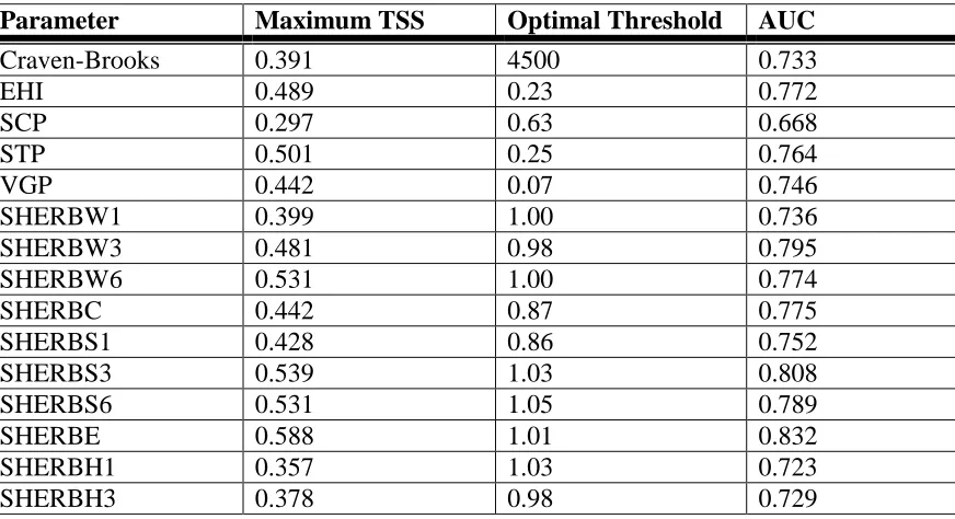
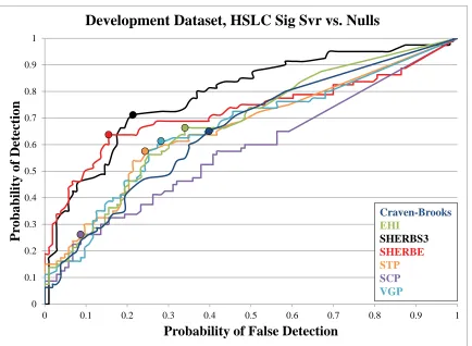
Table 3.2 Maximum true skill statistic (TSS), optimal threshold, and integrated area under the ROC curve (AUC) for given composite parameters at discriminating between HSLC significant severe reports and nulls within the development dataset. Composite parameters include the Craven-Brooks Significant Severe Parameter, Energy Helicity Index (EHI), Supercell Composite Parameter (SCP), Significant Tornado

Parameter (STP), and Vorticity Generation Parameter (VGP). ... 48

Table 3.3 As in Table 3.2, but for HSLC significant tornado reports and nulls. .... 49

Table 3.4 Maximum true skill statistic (TSS) using any threshold for (second column) all HSLC significant severe reports against nulls, (third column) HSLC significant tornadoes against nulls, (fourth column) HSLC significant winds against nulls, and (fifth column) HSLC significant hail reports against nulls within the nationwide verification dataset. ... 50

Table 3.5 As in Table 3.4, but for conventional parameter threshold values (Craven-Brooks: 20,000; EHI: 1; STP: 1; VGP: 0.2; SHERB

parameters: 1). ... 51

Table 3.6 Average cross- and along-boundary wind/shear components for high impact tornado days (HITOR) and high impact wind days (HIWND). .. 52

(10)

viii

List of Figures

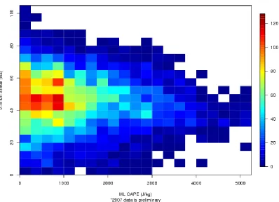
Figure 2.1 Tornado reports from 2003-2007 binned by MLCAPE and 0-6 km shear. From Schneider and Dean (2008). ... 18

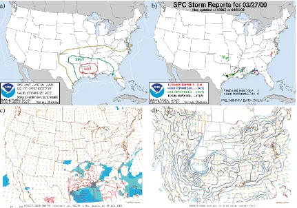
Figure 2.2 a) SPC 1300 UTC Day 1 Convective Outlook valid for 1300 UTC 27 March 2009 through 1200 UTC 28 March 2009; b) All severe weather reports from 1200 UTC 27 March 2009 through 1200 UTC 28 March 2009; c) SPC Mesoanalysis SBCAPE (J kg-1) field from 2000 UTC, the hour of the first tornado report in NC; d) as in c), but for 0-6 km shear magnitude (kt). ... 19

Figure 2.3 (left) 0.5 degree elevation plan position indicator radar reflectivity during 27 March 2009 mini-supercell HSLC event. White double arrow indicates a scale of 50 km. (right) Vertical cross section of mini-supercell at the center of left image. ... 20

Figure 2.4 Bow echo evolution as proposed by Fujita (1979). Arrows depict wind flow. The dashed line indicates the position of a system-generated cold pool. Solid contours and shading indicate areas of moderate and high values of radar reflectivity, respectively. Figure taken from Atkins et al. (2005). ... 21

Figure 2.5 Conceptual model of a trailing stratiform MCS. Arrows depict wind flow. The heavy black contour identifies the area of precipitation. Light and dark shading indicate areas of moderate and high values of radar reflectivity. Taken from Houze et al. (1989). ... 22

Figure 2.6 Case study evolution of a bow echo with mesovortices. Contours and shading are generally as in Fig. 2.4; the exception is dark shading indicating a straight-line wind damage swath associated with a strong, long-lived mesovortex. Circles with arrows indicate mesovortices. The thin, dark line during the bow echo stage shows the path of a tornado associated with a long-lived mesovortex relative to bow echo location. Taken from Atkins et al. (2005). ... 23

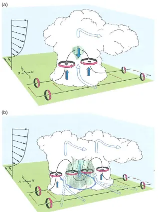
Figure 2.7 a) Initial development of counter-rotating mid-level vortices within a supercell as a result of the tilting of horizontal vortex lines by a

(11)

ix

vorticity. Blue filled arrows indicate regions of updraft (forced by perturbation pressure gradient forces) and downdraft, while unfilled arrows indicate low-level inflow and upper-level outflow. Green hatching indicates an area of precipitation. The blue line with triangles indicates the location of a storm-generated cold pool. Taken from

Markowski and Richardson (2010). ... 24

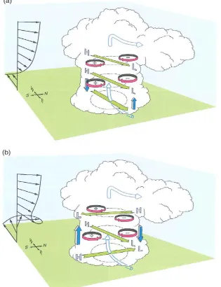
Figure 2.8 a) Perturbation pressure fields in a developing supercell within an environment with a straight hodograph; b) the same, but for a curved hodograph, producing preferential updrafts on the (storm motion-relative) right side of the supercell and downdrafts on the left side. Green arrows indicate shear vectors at the given levels. ―L‖ shows an area of low perturbation pressure, while ―H‖ represents an area of high perturbation pressure. Blue filled arrows indicate areas of updraft and downdraft forced by perturbation pressure gradient forces. Other symbols are as in Fig. 2.7. Taken from Markowski and Richardson

(2010). ... 25

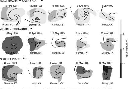
Figure 2.9 Cold pool virtual potential temperature perturbations (shaded) of observed significantly tornadic, weakly tornadic, and non-tornadic supercells. Black contours represent 40 dBZ radar reflectivity. Note the cooler temperatures (darker shading) in many non-tornadic and weakly tornadic cases. Taken from Markowski and Richardson (2009). ... 26

Figure 2.10 Resultant convective modes associated with three separate

environments, including varying wind and shear orientations relative to boundaries, during a case study of the 30 March 2006 severe

weather event. Taken from French and Parker (2008). ... 27

Figure 2.11 Top: All tornadoes occurring in environments with MLCAPE ≤ 500 J kg-1 between 2003-2009. Bottom: Same, but only including significant tornadoes (≥ EF2 on the enhanced Fujita scale). Taken from Guyer and Dean (2010). ... 28

Figure 2.12 Number of tornadoes occurring within a given hour from discrete cells and QLCSs during the (top) warm season and (bottom) cool season.

Taken from Thompson et al. (2008). ... 29

(12)

x

Figure 3.2 Nationwide distribution of all HSLC significant severe reports from

2006-2011 by NWS CWA ... 54

Figure 3.3 As in Fig. 3.2, but for only HSLC significant tornado reports. ... 55

Figure 3.4 As in Fig. 3.2, but for only HSLC significant wind reports. ... 56

Figure 3.5 As in Fig. 3.2, but for only HSLC significant hail reports. ... 57

Figure 3.6 Annual cycle of HSLC significant hail reports, significant wind reports, significant tornadoes, and nulls. ... 58

Figure 3.7 Annual cycles of a) all HSLC significant severe reports, b) HSLC significant tornado reports, c) HSLC significant wind reports, and d) HSLC significant hail reports by regions. e) Subjectively-defined regions as referred to in the text. Region labels: NW – Northwest; NR – Northern Rockies; NP – Northern Plains; UM – Upper Midwest; EGL – Eastern Great Lakes; NE – Northeast; SW – Southwest; FC – Four Corners; SP – Southern Plains; LMV – Lower Mississippi Valley; SA – South Atlantic. Colors in bar graphs correspond to region colors in e). ... 59

Figure 3.8 Diurnal cycle of HSLC significant severe reports and nulls by local solar hour where the report occurred. ... 61

Figure 3.9 Box-and-whisker plots showing the distributions of a) SBLCL, b) SBCIN, c) MUCAPE, and d) LLLR for all HSLC significant wind reports by region. Regions are defined in Fig. 3.7e. 25th and 75th percentiles are noted by the box, with the median noted by a horizontal line within the box. Whiskers extend to the 10th and 90th percentiles, and additional outliers are plotted as crosses. ... 62

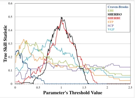
Figure 3.10 True skill statistic at discriminating between HSLC significant severe reports and nulls as a function of parameter threshold value for the given composite parameters in the development dataset. ... 63

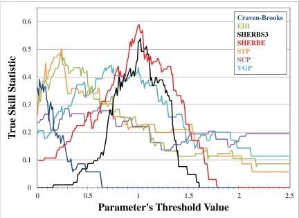
Figure 3.11 As in Fig. 3.10, but for HSLC significant tornadoes against nulls. ... 64

(13)

xi

Figure 3.13 As in Fig. 3.12, but for HSLC significant tornadoes and nulls. ... 66

Figure 3.14 Maximum true skill statistic for given composite parameters at discriminating between HSLC significant severe reports and nulls across all regions and entire U.S. Dots indicate those statistics calculated without including reports and nulls from collaborating county warning areas in regions 7 and 8, ensuring a truly independent dataset. Region SW is excluded due to a very low sample size. ... 67

Figure 3.15 SHERBS3 and SHERBE distributions for a) all significant HSLC events and nulls, b) significant HSLC tornadoes and nulls, c)

significant HSLC wind events and nulls, and d) significant HSLC hail events and nulls within the verification dataset. Plots are defined as in Fig. 3.9. ... 68

Figure 3.16 Θe differences across the given levels for reports and nulls. Here, a

positive difference indicates decreasing Θe with height. ... 69

Figure 3.17 Composite soundings for HSLC discrete supercells (DISC), supercells within clusters (CLUS), supercells within lines (LIN), and

non-supercells (NON) within the development dataset. Red, green, and blue lines on the skew-T/log-p show environmental temperature, environmental dew point temperature, and surface-based lifted parcel temperature, respectively. ... 70

Figure A1 Representative soundings taken from initialization of the DTDW simulation (blue) and NTNW simulation (red). The colored lines on the skew T-log p indicate environmental temperature (right) and dew point (left). Wind barbs are plotted for the DTDW simulation. All winds are storm-relative. Approximate values of SBCAPE and SBCIN are included for the given thermodynamic profiles (values across the two DT and two NT simulations vary slightly due to initial potential temperature perturbations). ... 101

Figure A2 Four-panel plots showing reflectivity (shaded), positive vertical velocity (green contours at 2.5, 5, 7.5, 10, 15, and 20 m s-1), and positive vertical vorticity (red contours at 0.01, 0.02, 0.03, and 0.04 s

-1_{) at 1 km and surface Θ perturbation of -1 K (blue dashed contours)}

(14)

xii

Figure A3 As in Fig. A2, but for t = 60 min. ... 103

Figure A14 Development of a strong, low-level vortex in DTNW simulation. Values in a) and b) are at approximately 1 km AGL, while values in c) and d) are from 25 m AGL. Panels a) and c) show vertical vorticity (10-3 s-1) shaded, with warm colors indicating positive values and cool colors indicating negative values. Updrafts and downdrafts are contoured at 1, 2.5, 5, 7.5, 10, 15, and 20 m s-1 in white and purple, respectively. Black, unfilled contours show quasi-reflectivity at 5 dBZ increments beginning at 40 dBZ. White, dashed contour shows potential temperature perturbation of -1 K. Vectors show total horizontal wind. Panels b) and d) show potential temperature perturbation (shaded), updrafts (white contours), downdrafts (magenta contours), and total horizontal wind vectors. The white arrow in d) shows the location of a cold pool surge, with white circles in c) noting the associated vortex couplet. ... 114

Figure A15 As in Fig. A2, but for the NOWCP run at t = 360 min. ... 115

(15)

xiii

vertical vorticity field representing values > 0.045 s-1. Note the relative strength of the surface cold pool compared to Fig. A14. ... 116

Figure A17 As in Fig. A1, but for DRY run. ... 117

Figure A18 As in Fig. A2, but for the DRY run at t = 150 min. ... 118 Figure A19 Development of strong, low-level vortices along outflow in NOWCPCOR

simulation. Fields are as in Fig. A14, with gray scale colors in the vertical vorticity field representing values > 0.045 s-1. ... 119

Figure A20 Development of strong vortex in DTNW high-resolution simulation. Fields are as in Fig. A14. Vortex of interest is located at approximately x = 0, y = -23 and noted by the white arrow. ... 120

(16)

xiv

List of Acronyms

ΔΘe: Equivalent potential temperature differences

Θ: Potential temperature

Θe: Equivalent potential temperature

AUC: Area under the ROC curve

CAPE: Convective available potential energy CIN: Convective inhibition

CLUS: Supercells within clusters

CM1: Cloud Model 1 (Bryan cloud model) CWA: County warning area

DISC: Discrete supercells

DRY: Simulation including dry intrusion DT: Discrete supercell thermodynamic profile

DTDW: Discrete supercell thermodynamic and wind profiles

DTNW: Discrete supercell thermodynamic profile and non-supercell wind profile DW: Discrete supercell wind profile

EF: Enhanced Fujita scale EGL: Eastern Great Lakes EHI: Energy Helicity Index EL: Equilibrium level ESHR: Effective shear FC: Four Corners

(17)

xv LCL: Lifted condensation level

LFC: Level of free convection LIN: Supercells embedded in lines LLLR: Low-level lapse rate LMV: Lower Mississippi Valley LR75: 700-500 hPa lapse rate MCS: Mesoscale convective system ML: Mixed-layer

MU: Most unstable NE: Northeast

NON: Linear non-supercells

NOWCP: Simulation with no initial winds in cold pool

NOWCPCOR: Simulation with no initial cold pool winds and Coriolis on perturbation winds

NOWCPDRY: Simulation with no initial cold pool winds and dry intrusion NP: Northern Plains

NR: Northern Rockies

NT: Non-supercell thermodynamic profile

NTDW: Non-supercell thermodynamic profile and discrete supercell wind profile NTNW: Non-supercell thermodynamic and wind profile

NW (body): Northwest

NW (Appendix): Non-supercell wind profile NWS: National Weather Service

POD: Probability of detection POFD: Probability of false detection QLCS: Quasi-linear convective system RIJ: Rear-inflow jet

(18)

xvi RUC: Rapid Update Cycle

S3MG: 0-3 km shear magnitude SA: South Atlantic

SB: Surface-based

SCP: Supercell Composite Parameter

SFCOA: Surface objective analysis (i.e., Mesoanalysis)

SHERB: Severe Hazards in Environments with Reduced Buoyancy parameter (derivatives defined in Table 3.1)

SP: Southern Plains

SPC: Storm Prediction Center SRH: Storm-relative helicity

STP: Significant Tornado Parameter SW: Southwest

TSS: True Skill Statistic UM: Upper Midwest

(19)

1

Chapter 1: Introduction

1.1 Motivation

The textbook severe weather environment in the United States—particularly that which is considered most conducive to tornadoes associated with supercells—is characterized by strong deep layer shear and significant convective available potential energy (CAPE; Schneider and Dean 2008). However, across the Southeastern and Mid-Atlantic states, environments with high shear1_{but low CAPE}2_{(HSLC) produce a substantial fraction of}

severe thunderstorms, including tornadoes (Schneider et al. 2006; Lane 2008; Schneider and Dean 2008; Guyer and Dean 2010). Schneider et al. (2006) referred to HSLC environments, coupled with low lifted condensation levels (LCLs; i.e., cloud bases), as the second ―key subclass‖ of severe weather in the U.S.

HSLC events tend to occur during the cool season or overnight (Burke and Schultz 2004; Guyer et al. 2006; Konarik and Nelson 2008; Smith et al. 2008; Kis and Straka 2010), when CAPE is at its minimum and shear is at its maximum climatologically, making them more likely to catch both forecasters and the public off-guard (Brotzge et al. 2011). In terms of annual trends, the cool season has a higher normalized fatality total than the late spring and early summer (Ashley et al. 2008), while the false alarm ratio for tornado warnings is relatively high compared to the rest of the year (Brotzge et al. 2011). Additionally, Schneider and Dean (2008) showed that the environment at any given location has less than 250 J kg-1 of mixed-layer (ML) CAPE ―the vast majority‖ of the time, meaning that HSLC environments contribute to a considerable amount of false alarm hours, while tornadoes

1_{Throughout the thesis, the term}_shear_{will be used in reference to the bulk shear vector magnitude over a}

layer.

2

(20)

2

occurring in HSLC environments are among the most often missed by Storm Prediction Center tornado watches (Dean and Schneider 2008; Dean and Schneider 2012).

Some areas in the Southeastern U.S. see large fractions of tornado-related fatalities and property damage occur with cool season events (Konarik and Nelson 2008). Meanwhile, Smith et al. (2008) showed that many of these events occur overnight, when the possibility of tornado deaths more than doubles (Ashley et al. 2008). Though the number of total tornado deaths has gradually decreased over the last five decades, nocturnal fatalities have seen a more subdued trend, leading to a higher relative percentage of nighttime tornado deaths (Ashley et al. 2008). These statistics suggest that the reported annual and diurnal trends of HSLC events tend to overlap with the highest relative risk to the public; however, a thorough investigation of warning verification statistics and storm-related casualties compared to environmental ingredients has not been performed.

(21)

3

example, may not be representative for HSLC events (Guyer and Dean 2010; R. Thompson 2012, personal communication), suggesting a diagnostic tool designed for environments with marginal instability may be operationally beneficial.

Observational investigation of HSLC events has been limited to the last two decades.

Case studies of severe HSLC events have noted a dry intrusion aloft may coincide with the onset of or strengthening of existing convection, perhaps indicating the release of potential instability (Johns 1993; Lane and Moore 2006; Clark 2009; Evans 2010), while modeling studies by McCaul and Weisman (2001) showed that in weak CAPE environments, more robust convection is possible when instability is focused in the lowest levels. Otherwise, recent studies have largely been focused on the operational utility of radar signatures such as the ―broken-S signature‖ (McAvoy et al. 2000; Grumm and Glazewski 2004; Clark 2011) and ―reflectivity tags‖ (Barker 2006). Despite some progress in radar operations, forecasting and nowcasting of HSLC events are still a challenge (Trapp et al. 2005; Schneider and Dean 2008; Dean and Schneider 2008). As indicated by McAvoy et al. (2000) and Lane and Moore (2006), relatively quick development of HSLC tornadic radar signatures such as those mentioned above result in low warning lead times. Meanwhile, quick storm motions along with the nocturnal nature of many events can provide difficulty for storm spotters, especially given the fact that some HSLC events have little to no cloud-to-ground lightning (Davies 1990; Cope 2004; van den Broeke et al. 2005; Schneider and Dean 2008). These unusual challenges during warning operations indicate a need for better understanding of the environmental ingredients associated with severe HSLC convection.

(22)

4

forecasters may alter their methods and foci depending on the convective mode. For instance, if discrete supercells are expected, forecasters will expect long-lived mid-level circulations which may lead to low-level circulations and subsequent tornadoes; however, in the case of quasi-linear convective systems (QLCSs), tornadic circulations are often shallow and confined to the lowest levels (Smith et al. 2012). Finally, and arguably most importantly, there is a need for greater understanding of the dynamics inherent to HSLC events. How do these events compensate for the relatively meager instability? What are the mechanisms for tornadogenesis in HSLC supercells and QLCSs? These are just a few of many unanswered questions regarding HSLC severe convection.

To address the operational and theoretical questions associated with HSLC severe convection, a statistical analysis was completed to compare databases consisting of HSLC severe convection and non-severe convection. In terms of operational HSLC considerations, conventional severe weather forecasting techniques were assessed, including a thorough comparison of the skill of various composite parameters. Moreover, environmental features that discriminate between events and nulls and also between differing convective modes were identified. These findings are meant to assist WFOs in preparation for and during forecast and warning operations for HSLC events. Combined with ongoing work meant to study HSLC convection through idealized simulations, these efforts allow for an improved understanding of how HSLC events work while exposing remaining uncertainties.

1.2 Thesis Structure

(23)

5

(24)

6

Chapter 2: Background

A broad spectrum of CAPE and shear combinations is capable of producing severe weather (Schneider and Dean 2008), representing a continuum within which any given environment lies (Fig. 2.1). As such, it is a challenge to define what is considered an HSLC environment. Previous studies have defined ―low CAPE‖ as MLCAPE of either ≤ 500 J kg-1 (Guyer and Dean 2010) or ≤ 1000 J kg-1 (Schneider and Dean 2008), while high 0-6 km shear thresholds have generally been ≥ 15 m s-1 or ≥ 18 m s-1 (Schneider and Dean 2006; Schneider and Dean 2008). By consensus among collaborating regional operational meteorologists, it was determined that suitable thresholds for HSLC events within this study were SBCAPE ≤ 500 J kg-1 and 0-6 km shear ≥ 18 m s-1. A representative case using these thresholds is shown through examples of the March 27, 2009 tornado outbreak across central and eastern NC (Fig. 2.2 and 2.3). Although widespread severe convection was not anticipated in NC by the Storm Prediction Center (SPC; Fig. 2.2a), 11 tornadoes occurred between 2000 UTC on 27 March 2009 and 0000 UTC on 28 March 2009 (Fig. 2.2b) in an environment characterized by SBCAPE of approximately 250 J kg-1 (Fig. 2.2c) and 0-6 km shear over 30 m s-1 (60 kt; Fig. 2.2d). These tornadoes developed in association with miniature supercells (Fig. 2.3), which will be explored in more detail shortly.

(25)

7

considered the most dangerous in terms of severe straight-line winds, while tornadoes have been postulated to occur just north of the apexes (Fig. 2.4; Fujita 1978, 1979, 1981; Atkins et al. 2005). Miniature supercells (hereafter, mini-supercells) are most common within HSLC and tropical environments. In general, mini-supercells are comparable in structure to classic supercells, though their spatial dimensions are compressed (Davies 1990; Kennedy et al. 1993; Smith et al. 2012). Tropical environments supporting mini-supercells consist of strongly curved hodographs, high moisture content, and relatively shallow and meager instability when compared to classic supercell environments (McCaul 1991; McCaul and Weisman 1996; Edwards et al. 2010). A thorough exploration of mid-latitude HSLC environments supporting mini-supercells has not been performed.

2.1 QLCSs

QLCSs are the ―linear‖ (i.e., squall line-like) subset of the broader phenomenon known as MCSs, which are regions of convective storms with unbroken horizontal extents of precipitation of at least 100 km (Glickman 2000). QLCSs are characterized by a region of deep convection and an associated region of stratiform precipitation, which can be found upstream from, parallel to, or downstream of the convection (Rotunno et al. 1988; Houze et al. 1989; Parker and Johnson 2000). The convective region consists of strong, episodic updrafts and is often associated with the greatest severe hazards; meanwhile, the stratiform region of precipitation occurs as a result of advection of hydrometeors as well as a weaker, mesoscale updraft which spreads out from the convective region (Rotunno et al. 1988; Houze et al. 1989). From regional case study investigations, trailing stratiform QLCSs were found to be the most common (Houze et al. 1990; Parker and Johnson 2000), although some other structures (i.e., parallel stratiform or leading stratiform) may be more frequently associated with severe hail and tornadoes (Gallus et al. 2008).

(26)

8

regions and a rear-to-front flow, which occurs at a lower elevation than (i.e., below) the front-to-rear flow (Fig. 2.5; Houze et al. 1989). The rear-to-front flow is a consequence of the pressure perturbations induced by the buoyant updraft and trailing anvil (Smull and Houze 1987). As a result, the strength of the rear-to-front flow is correlated with the strength of the QLCS, which can be augmented by increases in instability or line-relative wind shear (Weisman 1993). Both of these factors can promote vertically erect, sustained convection in QLCSs. As the rear-to-front flow approaches the convective region, it may be cooled and begin to descend, and this descending flow can result in an enhancement of surface winds (Houze et al. 1989; Mahoney et al. 2009). During the cool season, momentum transfer of strong winds from aloft has been noted to produce significant wind events, even in environments that are only marginally unstable (Johns 1993).

Recent observational studies (e.g., Funk et al. 1999; Lane and Moore 2006; Latimer and Kula 2010) have indicated that the rear-to-front flow, or rear inflow jet (RIJ) may play a key role in tornadogenesis during HSLC events. Atkins et al. (2005) suggested that tornadogenesis occurs coincident with the descent of the RIJ, which locally enhances the propagation speed of—and convergence along—the gust front. The strength of the RIJ may be associated with low-level shear, with some observational and idealized simulation studies suggesting a propensity for more intense, elevated RIJs in strongly sheared environments (e.g., Funk et al. 1999; Weisman and Trapp 2003), though this sensitivity is not well understood (Markowski and Richardson 2010). Further, the details of the relationship between the RIJ and HSLC tornadogenesis are unknown.

(27)

9

2003; Atkins et al. 2004; Atkins et al. 2005; Smith et al. 2010). Trapp and Weisman (2003) hypothesized that these mesovortices form as a couplet by the tilting of baroclinically-generated crosswise vorticity via a downdraft, with the cyclonic members becoming dominant over time due to the stretching of planetary vorticity (i.e., due to the Coriolis effect). The descent of the RIJ has been identified as a discriminating factor between significant and non-significant mesovortices, as it can be the necessary source of crosswise vorticity for downdraft tilting (Trapp and Weisman 2003; Atkins and St. Laurent 2009a). Atkins and St. Laurent (2009b) introduced the idea that cyclonic mesovortices could develop independently due to the procurement of downdraft-tilted baroclinic vorticity. Additionally, when vortex couplets were identified by Atkins and St. Laurent (2009b), they were formed by the tilting of crosswise baroclinic vorticity by the updraft along the gust front, rather than the downdraft, the latter of which had been suggested by Weisman and Davis (1998) and Trapp and Weisman (2003). Wheatley and Trapp (2008) noted that in their simulations of cool-season QLCSs, environmental horizontal vorticity is tilted into a vortex sheet, followed by the formation of mesovortices through shearing instabilities. No one theory has yet proven sufficient to encompass all potential genesis mechanisms of mesovortices.

The role of mesovortices in HSLC events has yet to be explored in great detail, despite observational evidence of their occurrence (e.g., Cope 2004). Though there have been documented cases of wind damage associated with mesovortices in non-HSLC events, many of these features are transient and do not produce any substantial effects (Atkins et al. 2004; Atkins et al. 2005). However, tornadoes or prolonged damaging winds can occur with mesovortices that are particularly long-lived and intense (Trapp and Weisman 2003; Weisman and Trapp 2003; Atkins et al. 2004; Atkins et al. 2005; Trapp et al. 2005; Wakimoto et al. 2006; Atkins and St. Laurent 2009a).

(28)

10

Laurent 2009a). In particular, as shear in the lowest 2.5 km increased, Weisman and Trapp (2003) showed deeper, sustained vortices extending upward to the mid-levels. This was a result of stronger environmental vorticity in the lowest levels, which acted to counter vorticity generated within the cold pool, leading to more vertically erect updrafts and thus more intense vortex stretching. Deep-layer shear seemed to play an overall less substantial role in the development of low-level mesovortices than did shear concentrated over the lowest few km, at least in high CAPE environments, because cold pools are confined to a relatively shallow layer (Weisman and Trapp 2003). Regardless of shear strength, the number of vortices increased with time in simulations (Weisman and Trapp 2003; Atkins and St. Laurent 2009a). Trapp and Weisman (2003) further noted that dominant cyclonic mesovortices did not develop in their simulations without the Coriolis force, the strength of which may also be relevant to the number of mesovortices produced (Atkins and St. Laurent 2009a). To the author’s knowledge, no previous studies have focused on the development and lifecycle of mesovortices within HSLC environments and how their strength and longevity is affected by limited buoyancy. Ongoing work will seek to address unanswered questions regarding the formation of mesovortices within HSLC convection through idealized simulations (reported in the Appendix).

2.2 Mini-Supercells

(29)

11

preferential updraft development on the right flank of the cell through perturbation pressure gradient accelerations (Fig. 2.8). The low-level mesocyclone is subsequently formed through the tilting of storm-generated baroclinic vorticity produced by the supercell’s downdraft. For tornadogenesis to occur, it is believed that tilting and convergence along the rear-flank downdraft concentrates vertical vorticity near the surface. This vorticity can then be stretched into a tornado (Markowski and Richardson 2010).

Despite being shallower and often weaker (in terms of updraft strength) than classic supercells, discrete mini-supercells have been shown to be associated with strong mesocyclones (Edwards et al. 2010). In their simulations, McCaul and Weisman (1996) showed that low-level mesocyclone strength in mini-supercells is correlated to the temperature of the storm’s cold pool, which has been shown to be relevant to likelihood of tornadogenesis in non-HSLC supercells in previous studies, as depicted in Fig. 2.9 (e.g., Markowski et al. 2002; Markowski and Richardson 2009). McCaul and Weisman (1996) suggested that relatively warm cold pools in tropical mini-supercells were a reason for their associated weak tornadoes, whereas Markowski et al. (2002) suggested that warmer cold pools were typically associated with stronger tornadoes. This indicates a possible ―Goldilocks‖ scenario in which strong tornadoes can only form given a certain range of cold pool temperature—not too cool or too warm. If the cold pool is too cool, cold pool air will be too negatively buoyant to be lifted and stretched by the updraft. However, if the cold pool has a comparable temperature to inflow air, the baroclinic production of horizontal vorticity will be insufficient for subsequent tornado development through tilting and stretching (Markowski et al. 2002).

(30)

12

vertical accelerations due to buoyancy are similar to those resulting from dynamic pressure perturbations, suggesting a heightened importance for favorable dynamic pressure perturbations in HSLC environments (McCaul and Weisman 1996).

McCaul and Weisman (2001) showed through supercell simulations that storm strength is influenced by the vertical distribution of CAPE, with higher concentrations of CAPE in the low levels corresponding to more intense convection. In a more recent study, Lane (2008) also indicated that the vertical distribution of CAPE may be a factor in determining likelihood of tornadogenesis in HSLC cases. McCaul (1991) found similar trends in tropical low CAPE environments, as static stability below 700 hPa (approximately 3 km) was weak in tornado events compared to Oklahoma supercell composite soundings. Additionally, though precipitable water values are comparable between high and low CAPE severe events (Guyer and Dean 2010), many previous studies (e.g., Schneider et al. 2006; Schneider and Sharp 2007; Guyer and Dean 2010) indicate the prevalence of low LCLs and high low-level moisture content in low CAPE tornado environments. Furthermore, severe HSLC environments (particularly those associated with tornadoes or damaging winds) are often characterized by substantial curvature in low-level winds, leading to large values of storm-relative helicity (SRH), which is generally proportional to the amount of streamwise vorticity that can be ingested by a supercell (e.g., Cope 2004; Wasula et al. 2008; Guyer and Dean 2010; Latimer and Kula 2010). Even in low CAPE environments that are marginally unstable throughout the depth of the troposphere, dynamically-driven strong updrafts near the surface may provide maximum potential for tilting and stretching of this environmental SRH along with storm-generated vertical vorticity, leading to the development of mesocyclones, mesovortices, and/or tornadoes.

2.3 Convective Mode Forecasting

(31)

13

(32)

14

2.4 Existing Climatologies

2.4.1 HSLC Tornadoes

Guyer and Dean (2010) provided a general overview on tornadoes forming in marginally unstable environments. As in this study, Guyer and Dean (2010) used a threshold of 500 J kg-1 to distinguish low CAPE environments, though they chose to utilize MLCAPE rather than SBCAPE. Over one-quarter of all tornado reports during their time period of study occurred in low CAPE environments and a considerable fraction of these tornadoes were significant (Fig. 2.11). Between December and February, low CAPE tornadoes accounted for over half of all tornadoes, supporting the notion of their relative commonality during the cool season (Guyer et al. 2006). When comparing the environments of low CAPE and high CAPE tornadoes, it has been shown that SRH and low-level moisture content are generally higher in lower CAPE environments (Schneider et al. 2006; Konarik and Nelson 2008; Guyer and Dean 2010; Latimer and Kula 2010). However, despite the handful of studies exploring tornadoes occurring in low CAPE environments, a comprehensive investigation into the climatology of HSLC tornadoes and the features unique to their environments embodies a current gap in the knowledge base.

2.4.2 QLCSs

(33)

15

tornadoes are maximized (Trapp et al. 2005; Thompson et al. 2008; Smith et al. 2010). Previous studies (e.g., Knupp et al. 1996; Konarik and Nelson 2008) have shown that some locations in the South get a substantial fraction to even a majority of their tornadoes from QLCSs, though that is subject to the chosen classification method (e.g., Smith et al. 2012). Additionally, though tornadoes are often the main concern to public and forecasters, QLCSs are also commonly associated with high impact straight-line wind events (Smith et al. 2010).

The frequency of QLCSs within HSLC environments is noted in the literature (e.g., Burke and Schultz 2004; Reilly 2004; Latimer and Kula 2010). Thus, the threat of HSLC QLCSs has been acknowledged, and the correlation between the diurnal and annual cycles of QLCSs and HSLC environments cannot be understated. However, as noted previously, a comprehensive investigation of HSLC events has not been completed prior to this study.

2.4.3 Mini-Supercells

(34)

16

2.5 Unanswered Questions Addressed in This Study

2.5.1 HSLC Climatology

As noted in the preceding discussion, a comprehensive climatology of HSLC events is not provided in the literature. One facet of this study will be to fill this knowledge gap, focusing on regional, annual, and diurnal variations in HSLC significant severe weather. Previous research (e.g., Dean and Schneider 2008) and personal discussion with NWS forecasters indicate that HSLC events pose a unique challenge to operations, both in forecasting and nowcasting (i.e., warning operations). Conventional techniques and composite forecasting parameters struggle to adequately represent the threat in marginally unstable environments. This study will address such difficulties through a detailed statistical analysis of environments associated with HSLC significant severe (i.e., tornadoes ≥ EF2, wind gusts ≥ 65 kt, and hail ≥ 2‖ in diameter) events compared to non-severe HSLC convection. Of particular concern will be to identify what environmental parameters discriminate most skillfully between the two types of convection. Additionally, previous studies have observed a dependency of convective mode on the orientation of deep-layer shear and winds relative to boundaries in high shear, high CAPE environments. This study will include a brief investigation into how these relative orientations affect both storm morphology and hazard type in HSLC situations.

2.5.2 Dynamical Understanding

(35)

17

(36)

18

(37)

19

Figure 2.2. a) SPC 1300 UTC Day 1 Convective Outlook valid for 1300 UTC 27 March 2009 through 1200 UTC 28 March 2009; b) All severe weather reports from 1200 UTC 27 March 2009 through 1200 UTC 28 March 2009; c) SPC Mesoanalysis SBCAPE (J kg-1) field from 2000 UTC, the hour of the first tornado report in NC; d) as in c), but for 0-6 km shear magnitude (kt).

a) b)

(38)

20

Figure 2.3. (left) 0.5 degree elevation plan position indicator radar reflectivity during 27 March 2009 mini-supercell HSLC event. White double arrow indicates a scale of 50 km. (right) Vertical cross section of mini-supercell at the center of left image.

(39)

21

(40)

22

(41)

23

(42)

24

(43)

25

(44)

26

(45)

27

(46)

28

(47)

29

(48)

30

Chapter 3: Parameter-Based Climatology

The first focus of this research was to improve the forecasting of high shear, low CAPE (HSLC) significant severe weather. More specifically, this study focuses on identifying environmental features that skillfully discriminate between HSLC significant severe convection and non-severe convection. This began with a basic climatology of HSLC significant severe weather, which is a current gap in the knowledge base. The long range goal was to address the void in HSLC operational techniques through statistical analysis. What environmental parameters are most relevant in discriminating between an HSLC significant severe event and a non-severe event? Can we improve current forecasting techniques and parameters or perhaps develop new techniques to address this unique challenge? Are there any tips for forecasting convective mode or potential hazards that can be reaped from existing data? These questions were addressed in the climatology phase of this study.

3.1 Climatology Data and Methods

3.1.1 Development Data – Events

Because HSLC severe weather is one of the most common challenges for forecasters in the Southeastern U.S. (Dean and Schneider 2012; J. Lane and P. Moore 2012, WFO Greenville-Spartanburg, personal communication), we began by creating a development (or ―training‖) dataset for this region. Collaborators from 11 National Weather Service (NWS) Weather Forecast Offices (WFOs) across the Southeast and Mid-Atlantic3 subjectively compiled a

3

(49)

31

list of HSLC events in their respective county warning areas (CWAs) between fall 2006 and spring 2011. HSLC events were defined as those with surface-based (SB) CAPE ≤ 500 J kg

-1

and 0-6 km shear ≥ 18 m s-1. The Storm Prediction Center (SPC) provided a relational database consisting of well-known convective environmental parameters for the 6245 severe reports that occurred in the collaborating CWAs during the 107 identified events. For each report, the relational database included the archived surface objective analysis4 (SFCOA; Bothwell et al. 2002) value for 90 standard parameters at the nearest grid point for the preceding hour. Additionally, convective mode classification was provided for most significant wind, significant hail, and tornado reports (see Smith et al. 2012 for additional information).

Because the SPC relational database included all regional reports between the given start and end times for each event, a large percentage of the reports in the database were not actually HSLC reports, as determined by the SFCOA data. For our formal analysis, we only retained a particular CWA’s reports for an event if over half of those reports met the HSLC

criteria defined above. Events fulfilling these criteria in one or more CWAs were designated as ―HSLC events.‖ In order to prevent dataset bias towards individual events with

particularly widespread reports, only one report was retained per CWA per hour. Tornadoes had the highest priority in this filtering process, followed by wind and hail reports, respectively. In other words, a wind report was used if there were no tornadoes in the CWA during that hour, while a hail report was used if there were no wind reports or tornadoes in the same CWA for a given hour. Each report type was subsequently sorted by magnitude prior to filtering (in other words, an EF3 tornado on the enhanced Fujita scale would take precedence over an EF2 tornado if both occurred in the same CWA and hour). The final, filtered dataset consisted of 943 reports (one per CWA per HSLC hour), including 80 significant reports (35 significant tornadoes, 44 significant wind reports, and 1 significant hail report). Through discussion with NWS and SPC collaborators, it was decided that the most operationally beneficial comparison would be between significant severe reports (i.e.,

(50)

32

tornadoes ≥ EF2, wind gusts ≥ 65 kt, and/or hail ≥ 2‖ in diameter) and nulls (defined next).

This approach helps to avoid some of the potential non-meteorological factors associated with severe but non-significant reports (e.g., Weiss et al. 2002; Doswell et al. 2005; Trapp et al. 2006), giving us higher confidence in our own development dataset.

3.1.2 Development Data – Nulls

(51)

33 3.1.3 Verification Dataset

After an initial assessment of environmental parameters, an independent5 verification dataset of reports and nulls was necessary to test our findings. For this purpose, the SPC produced a second relational database consisting of all significant severe reports and null points across the contiguous U.S. from 2006-2011 (nulls began in Oct. 2006 due to missing data in the archive). In this relational database, the data for both the events and nulls were gathered using the nearest data point from the preceding hour’s SFCOA. Only reports and

nulls meeting our HSLC criteria of SBCAPE ≤ 500 J kg-1 and 0-6 km shear ≥ 18 m s-1 were utilized in verification in addition to the climatology results of Section 3. Overall, the verification dataset included 2517 HSLC significant severe reports—302 tornadoes, 1579 wind reports, and 636 hail reports—and 1316 HSLC nulls.

3.1.4 Suitability of SFCOA

Arguably the main concern with the data used for this project is its reliance on model fields rather than observations. Though the SFCOA ingests surface observations, upper air features are dependent on fields from the Rapid Update Cycle (RUC) model; thus, biases and errors are common, as documented by Thompson et al. (2003) and more recently by Coniglio (2012). In addition, the SFCOA resolution is less than ideal, with 40 km horizontal grid spacing and archived data available only once every hour. This could lead to smoothing or misplacement of significant mesoscale features. Additionally, using the nearest grid point could occasionally result in the sampling of a different air mass if the report occurred close to a boundary.

5

(52)

34

Despite its limitations, the SFCOA markedly improves on RUC analyses, significantly reducing errors when compared to observations (Coniglio 2012). Further, using SFCOA fields rather than proximity soundings vastly increases the sample size and resolution of our datasets. Additionally, prior climatological studies (e.g., Thompson et al. 2007) utilized SFCOA data, so there is consistency between existing operational literature and the present study. Finally, through personal communication with forecasters at numerous WFOs, it became clear that SFCOA fields are commonly used during operations. Therefore, the data utilized for this study appear to be appropriate for an operationally-driven study. A more thorough discussion on utilizing the SFCOA for research was provided by Thompson et al. (2012).

3.1.5 Statistical Methods

Environments of HSLC significant severe reports and null points within the development dataset were compared via statistical analyses, focusing on parameters that showed high probability of detection (POD) and a low probability of false detection (POFD; Doswell et al. 1990). The True Skill Statistic (TSS; Wilks 1995) was utilized in order to determine which environmental parameters in the relational databases were most skillful at discriminating between events and nulls. The TSS is defined by

(1),

(53)

35

possibilities (a-d) in the standard contingency table (Fig. 3.1), including correct nulls (a category that is not practical for studies of warning verification, for example). We view the inclusion of correct nulls as particularly important because a forecaster must be able to trust a parameter when it predicts a non-event in addition to when it predicts an event. Finally, previous parameter-based studies (e.g., Thompson et al. 2004b) have utilized the TSS for determining the optimal value of composite parameters such as the Significant Tornado Parameter (STP). Receiver operating characteristic (ROC; Metz 1978) curves in addition to the integrated area under the ROC curve (AUC) were calculated as another measure of skill. Values of the AUC range from 0 to 1, with AUC < 0.5 representing negative skill (worse than a chance forecast), AUC = 0.5 representing equivalent skill to a chance forecast, and AUC = 1 signifying a perfect forecast (Marzban 2004). Heidke Skill Scores (HSS; Wilks 1995) were also calculated, and trends were generally similar to those of the TSS and AUC. HSS values tended to diverge from the TSS in situations where the sample sizes of events vs. nulls differed considerably. In these cases, the TSS tended to value high POD, while the HSS preferred low false alarm ratios.

(54)

36

tests, only 10 reports and nulls were used for the last round. These tests largely confirmed the original findings (i.e. the same environmental parameters had the highest average TSS across all simulations in the respective round), except in the case of the third conditionally most skillful environmental parameter, for which there were a number of nearly equal options. In developing our composite diagnostic parameters, we considered each of these nearly equal third ingredients in turn, as described and assessed in Section 3.2.2.

After the initial assessment of environmental parameters in our Southeastern U.S. development dataset, the independent nationwide verification dataset of reports and nulls (Section 3.1.3) was used to test the robustness of our findings. To test regional and nationwide applicability of the results from the development dataset, the TSS was again used. Additionally, two-sample t-tests (Wilks 1995) were administered and their associated

p values were calculated in order to assess the statistical significance of differences in means between the reports and nulls datasets.

3.2 HSLC Climatology

3.2.1 Diurnal, Annual, and Regional Trends

(55)

37

(Fig. 3.5). Some local maxima and minima are likely attributable to non-meteorological factors associated with differing local warning verification techniques (e.g., Doswell et al. 2005), but the transition from a wind and tornado threat across the Southeastern U.S. to primarily wind and hail reports across the Plains and Upper Midwest likely is

meteorological, as will be explored shortly.

Annually, both HSLC significant severe reports and nulls have an April peak, followed by a decrease through the summer and early fall with only a weak secondary maximum in October (Fig. 3.6). December was the only month with a higher number of nulls than significant reports, suggesting a decrease in warning skill during that month (although the sample size is rather small compared to most other months). When breaking the annual cycle down by subjectively defined regions (see Fig. 3.7e), many similarities to previous climatologies of severe weather (e.g., Brooks et al. 2003; Doswell et al. 2005) became evident (Fig. 3.7a). Fall and winter (September-February) HSLC significant severe reports predominantly occurred in the South Atlantic and Lower Mississippi Valley regions. In the spring (March-May), reports became increasingly common in the Southern Plains and the Upper Midwest. By summer (June-August), the Northern Plains accounted for a large fraction of HSLC significant severe reports. HSLC significant tornado reports (Fig. 3.7b) have a February-April maximum in the Lower Mississippi Valley and South Atlantic, accounting for most of the overall distribution shown in Fig. 3.3 and consistent with the annual cycle of Guyer et al. (2006). A clear annual minimum in HSLC tornadoes occurred in the summer, presumably because CAPE is typically high and shear is typically low over much of the U.S. The HSLC significant wind reports (Fig. 3.7c) have similar trends to the total HSLC significant reports (cf. Fig. 3.7a), largely because the majority of HSLC reports are winds. The HSLC significant hail threat (Fig. 3.7d) was largely nonexistent through the winter, with a rapid increase in spring. As with severe winds, by summer, the threat was primarily in the Plains and Upper Midwest.

(56)

38

minimum. Notably, false alarms (nulls) were proportionally larger during the overnight and morning (the null counts roughly equal or surpass significant severe reports from 0300-1000 local solar time). This finding is consistent with previous work on tornado false alarms by Brotzge et al. (2011).

Given these regional differences in timing and in predominant HSLC severe weather type, we studied the typical values of environmental parameters in significant wind events by region. Here, only wind events were utilized to prevent the complicating factor of comparing tornado, wind, and hail environments. It became apparent that there are likely multiple U.S. regimes of HSLC severe weather. HSLC environments east of the Mississippi River (the EGL, NE, LMV, and SA regions) tended to have similar low-level moisture content (LCL height) but smaller (less negative) SB convective inhibition (CIN) than reports in the Plains and Midwest (the NP, SP, and UM regions), as shown in Figs. 3.9a and 3.9b. The larger SBCIN, combined with rather large most unstable (MU) CAPE values (Fig. 3.9c), suggests that many HSLC events in the Plains and Midwest may have actually occurred with elevated—rather than SB—convection. It also appeared that some HSLC events may be high-based storms in environments with dry boundary layers. There were a considerable number of reports in the dataset with SB LCLs near or above 1 km (Fig. 3.9a), especially in the Northern Rockies (NR) and Northwest (NW) where steep low-level lapse rates prevail (Fig. 3.9d). It is likely that environments for elevated or high-based convection are considerably different from the moist, surface-based HSLC environments of the Southeastern U.S., from which our development dataset was drawn. We explore the possibilities and limitations of a ―one size fits all‖ HSLC composite parameter in the next

section.

3.2.2 Development of an HSLC Composite Parameter

(57)

39

severe convection (tornado, winds, and hail) and nulls in the development dataset were the 0-3 km lapse rate (i.e., low-level lapse rate or LLLR) and the 700-500 hPa lapse rate (LR75). The third conditionally most skillful parameter was less well defined due to a vastly decreased sample size in the third round of TSS tests. The initial TSS tests and subsequent Monte Carlo simulations revealed a number of wind and shear parameters that have comparable skill (listed in Table 3.1).

On its own, LLLR had the highest skill among tested parameters with a maximum TSS of 0.342. This value exceeded the TSS of even well-known composite parameters (the STP was the best of them with a TSS of 0.332). Through the procedure in Section 3.1.5, it was further determined that by utilizing LR75 as the second parameter in tandem with LLLR, the TSS increased to 0.463. Due to the assortment of wind and shear values that were roughly equal as the third most conditionally skillful ingredient, composite parameters consisting of products of the LLLR, LR75, and each wind/shear metric were created. Each environmental parameter was normalized by its optimal threshold value (i.e., the threshold at which its skill was maximized; the normalization of the wind/shear term was adjusted slightly in order to produce an optimal value of 1 for the final composite parameter within the development dataset). As shown in Table 3.2, the most skillful composite parameter within our development dataset (at discriminating between HSLC significant severe reports and nulls) was the version of the Severe Hazards in Environments with Reduced Buoyancy parameter using the 6 km wind magnitude (or SHERBW6; this and other abbreviations are given in Table 3.1). This was also reflected in the integrated metric of area under the ROC curve (AUC) for each parameter.

(58)

40

formulations remained especially skillful (SHERBE, SHERBW3, SHERBS3, SHERBW6, SHERBS6), while the aforementioned low skill formulations were again poor discriminators; as such, they were removed from consideration for our subsequent analysis6. By utilizing the nationwide verification dataset, it became apparent that the SHERBE and SHERBS3 were the most skillful SHERB parameters. Table 3.4 shows the maximum TSS in discriminating between HSLC significant severe reports and nulls (also divided into tornado, wind, and hail reports vs. nulls), using the threshold that maximized the TSS for each individual parameter. More telling were the skill scores using the parameters’ conventional thresholds, shown in Table 3.5. These statistics revealed that the SHERBE was the best performing composite parameter within the nationwide HSLC verification dataset. While SHERBS3 and SHERBE optimal thresholds were consistent across most subsets, the thresholds of conventional composite parameters must be adjusted downward to maximize their skill (see Fig. 3.10). At their normal thresholds, SHERBS3 and SHERBE also outperformed all conventional parameters at separating tornadoes from nulls in the development dataset (Fig. 3.11). ROC curves show similar trends (Fig. 3.12 and Fig. 3.13). As a result, the remainder of Section 3.2.2 will focus on assessing the skill of these two parameters.

The SHERBE, or the Severe Hazards in Environments with Reduced Buoyancy Parameter (using effective7 shear, or ESHR) is specifically formulated as

SHERBE = (ESHR / 27 m s-1) * (LLLR / 5.2 K km-1) * (LR75 / 5.6 K km-1).

Although SHERBE was the most skillful parameter, we noted that some HSLC significant severe reports occurred in environments with diagnosed MUCAPE of 0 J kg-1 in the SFCOA. This is problematic because ESHR is by definition 0 m s-1 when there is no CAPE

6

All of the parameters listed in Table 3.1 were subjected to the same tests as the parameters referenced hereafter. For sake of clarity and brevity, only chosen parameters were included in subsequent figures, tables, and discussion.

7_{The effective shear magnitude is calculated from the most unstable parcel’s lifted level upward through half}

(59)

41

(Thompson et al. 2007), which would in turn cause SHERBE to be 0. Therefore, as a practical consideration, we also tested the most skillful fixed-layer version of the SHERB, which was formulated using the 0-3 km shear magnitude (S3MG),

SHERBS3 = (S3MG / 26 m s-1) * (LLLR / 5.2 K km-1) * (LR75 / 5.6 K km-1).

When testing across all nationwide HSLC significant severe reports, it becomes clear that the skill of SHERBS3 and SHERBE has noteworthy regional variations, as do all composite parameters (Fig. 3.14). In the regions that included our collaborating CWAs (i.e., LMV and SA, part of which made up our development dataset), the skill is high, as anticipated. Even without including our collaborating CWAs in the verification, the skill in these regions remains elevated compared to other composite parameters, as shown by the filled circles in Fig. 3.14. There are also multiple other regions, including the Eastern Great Lakes, the Northern Rockies, the Northwest, the Southern Plains, and the Four Corners region in which either the SHERBS3 or SHERBE shows the highest skill at discriminating between HSLC significant severe convection and nulls. In all but the Southwest, two-sample t-tests reveal that the differences in SHERBS3 between the significant severe reports and nulls are statistically significant at the 0.95 level (for the SHERBE, this is true in the NP, UM, EGL, SP, LMV, and SA regions). Despite regional skill variability, distributions of SHERBS3 and SHERBE values for nationwide events and nulls show reasonable separation, particularly for significant tornado events vs. nulls (Fig. 3.15).

(60)

42

the original development of ESHR by Thompson et al. (2007) was partially inspired by the knowledge that, for shallow storms (such as those in HSLC cases), conventional fixed-layer shear parameters were found to be unrepresentative (i.e., because a conventional fixed layer constituted too great a fraction of the overall storm depth). Meanwhile, low-level shear magnitudes such as the S3MG have been identified as discriminators between severe and non-severe convection, particularly in cases of QLCS mesovortices and tornadoes (Weisman and Trapp 2003; Godfrey et al. 2004; Lane and Moore 2006), which are common in HSLC environments (Davis and Parker 2012).

3.2.3 Comparison of SHERBS3/E to Other Composite Parameters in HSLC

Environments