Material Effects and Tool Wear in Vibration Assisted Machining.

(1)

ABSTRACT

LANE, BRANDON MICHAEL. Material Effects and Tool Wear in Vibration Assisted Machining. (Under the direction of Thomas Dow.)

Certain materials such as steels, nickel, and titanium alloys cause rapid thermo-chemical tool wear and poor surface finish during conventional diamond turning (DT). Optical quality surface finishes on these materials are possible when vibration-assisted machining (VAM) is incorporated. It is theorized that VAM reduces tool wear by reducing tool temperatures and forces. The goal of this research is to observe and measure tool wear during VAM and identify how this wear is related to process parameters, and how it is mitigated with VAM.

Baseline conventional DT tests on thermo-chemical wearing material were carried out in conjunction with finite element (FE) simulations of the DT process to develop a thermo-chemical wear model. To relate this model to VAM, kinematic calculations were made identifying related parameters; namely relative tool tip velocity and uncut chip thickness. FE simulations of the elliptical vibration assisted machining (EVAM) process are carried out that vary input EVAM parameters. Tool temperatures are extracted from FE data and supplied to the thermo-chemical wear model. These predictions are used to identify optimal EVAM conditions to minimize thermo-chemical wear.

(2)

Material Effects and Tool Wear in Vibration Assisted Machining

by

Brandon Michael Lane

A dissertation submitted to the Graduate Faculty of North Carolina State University

in partial fulfillment of the requirements for the Degree of

Doctor of Philosophy

Mechanical Engineering

Raleigh, North Carolina 2012

APPROVED BY:

_______________________________ ______________________________

Thomas A. Dow Ronald. O. Scattergood

Chair of Advisory Committee

(3)

BIOGRAPHY

Brandon Lane was born in Reno, Nevada, in 1984 and grew up in a small town in central Nevada called Battle Mountain, accurately dubbed by the Washington Post as “The Armpit of America”. After graduating at Battle Mountain High School, he then pursued a degree in Computer Science at University of Nevada, Reno. After determining that disdain for program debugging contributed to an unhealthy skiing addiction, he joined the Mechanical Engineering department at UNR. He spent his summers working for the Bureau of Land Management as a ground traffic controller for wildland firefighting airtankers or as a grunt on a fire engine.

Increased focus on engineering led him to an internship with the R&D department Hamilton Company in Reno, which designs and manufactures automated fluid-handling devices for medical and biological research purposes. He also was elected as the Vice President of the UNR chapter of Society of Women Engineers after succumbing to persuasion from his female engineering friends. He was also awarded an NSF-EPSCoR undergraduate research grant at UNR, and helped develop carbon-based nano-composite manufacturing techniques with Dr. Jonghwan Suhr at the Multifunctional Nano-Composite Lab.

(4)

(5)

ACKNOWLEDGMENTS

Special thanks to my family for putting up with a son/brother that is thousands of miles away, and is often too busy to remember to call.

Special thanks to Dr. Dow for providing the opportunity, facilities, and mentorship required for a successful graduate career. He provided invaluable lessons on better communication and its requirement for success.

Thanks to Alex Sohn and Ken Gerrard as invaluable resources of experience at the PEC. Erik Zdanowics, Guillaume Robichaude, John Nowak, and Zack Marston provided the most entertaining and friendly work environment possible. Thank you for not filing complaints for all the practical jokes.

A very special thanks to Benjamin Bulla, Sophia Hannig, Arne Matrose, and Christian Wenzel at Fraunhofer IPT in Aachen, Germany for hosting Dr. Dow and myself and providing us with time, facilities, and expertise. They provided facilities and equipment for all the ultrasonic machining experiments mentioned in Chapter 6. They cannot be thanked enough.

(6)

TABLE

OF

L

IST OF

T

ABLES

Table 5-1: Machining parameters for initial FE model of EVAM ... 103

Table 5-2. Simulation parameters for 4 EVAM and 4 conventional cutting simulations .... 113

Table 5-3. Machining parameters for 3 EVAM-FEM models varying ellipse shape. ... 118

Table 5-4: Simulation parameters for 4 EVAM simulations varying frequency ... 124

Table 5-5: Simulation parameters for 3 EVAM simulations increasing frequency while decreasing horizontal amplitude ... 129

Table 5-6: Simulation parameters for 4 EVAM simulations varying frequency and reduced ½ the amplitude ... 134

Table 6-1. EVAM machining parameters for cutting experiments varying frequency ... 148

Table 6-2: Operating conditions for 80 kHz Son-X device that achieve 20% duty cycle. ... 176

Table 6-3: Son-X machining parameters for AISI1215 tests ... 178

Table 6-4: Wear results for AISI1215 ultrasonic machining experiment ... 183

Table 6-5: Machining parameters for ultrasonic machining of Stavax flat ... 186

Table 6-6: Wear results for ultrasonic machining of Stavax flats ... 196

Table D-1: High-speed conventional DT of AISI1215. DoC= 1μm. 1.2mm wide workpiece. 235 Table D-2: Mid-speed conventional DT of AISI1215. DoC = 1μm. 0.25 mm wide workpiece Note the negative values for characteristic wear depth per cut distance ... 235

Table D-3: Low-speed conventional DT of AISI1215. DoC = 1μm. 0.25 mm wide workpiece ... 236

Table D-4: EVAM multi-frequency experiments with Ultramill on AISI1215. Depth of cut was 2 μm for each cut. ... 237

Table D-5: EVAM multi-ellipse experiment with Ultramill on AISI1215. Depth of cut was 10 μm for each cut ... 237

(12)

L

IST OF

F

IGURES

Figure 1-1: Schematics of 1D linear vibration assisted machining (LVAM, left) and 2D

elliptical vibration assisted machining (EVAM, right)[52]. ... 7

Figure 2-1: Schematic of 1D cutting tool wear measures on a round tool... 12

Figure 2-2: Schematic of different definitions of ‘wear area’ on a round tool. ... 14

Figure 2-3: Schematic showing wear area defined by Thornton and Wilks [27,66]. ... 14

Figure 2-4: Wear area defined by Durazo-Cardenas et. al. is area of edge recession along rake face [12]. ... 15

Figure 2-5: Microphotograph of rake face and flank face of round diamond tool from [72]. ‘Upper boundary’ indicates region nearer the feed direction. ... 18

Figure 2-6. Top Left: Viewing angle of EBID stripe on the diamond edge. Top Right: Example EBID image. Bottom: Worn area and cross-section measurement via Matlab script. 22 Figure 2-7: Wear rate (wear area / machined surface area in 10-6 mm2/mm2) of single crystal diamond tool as a function of air pressure at cutting speed of 0.013 mm/s (left) and 0.13 mm/s (right) [27]. Curve and transition range are added for clarity. ... 28

Figure 2-8: SEM image of diamond tools after CT and EVAM of W2 tool steel [52] ... 35

Figure 2-9: Diamond tool wear results from CT of AISI1045 steel baseline tests performed by Brinskmeier et. al. [35]. Machining distance for each test is 12 m. ... 36

Figure 2-10: Diamond tool wear results from EVAM of AISI1045 steel baseline tests performed by Brinskmeier et. al. [35]. AFM tool wear measurement (left) is after 1500 m machining distance. ... 37

Figure 2-11: Left: Schematic of Song et. al.’s fly-cutting tool wear experiment [119]. Right: Tool wear vs. contact time results after 100mm cumulative cutting distance. Some convexity width values are calculated from the plot and added for clarification. ... 42

(13)

Figure 3-2: Results from Matlab surface fit tool (sftool) relating temperature rise to workpiece speed and depth of cut obtained from FE models. R2 correlation was

0.998. ... 55

Figure 3-3: Multi-speed machining experiment setup for three speed ranges ... 57

Figure 3-4: Cutting zones on straight-edged diamond tool used in low and mid-speed orthogonal cutting experiments. ... 58

Figure 3-5: Worn tool cross-sections for high speed cutting experiments ... 59

Figure 3-6: Worn tool cross-sections for mid-speed cutting experiments ... 60

Figure 3-7: Worn tool cross-sections for low speed cutting experiments ... 60

Figure 3-8: EBID cross sections of worn tool edges comparing wear at mid speed and low distance vs. wear at high speed at large distance. ... 61

Figure 3-9: EBID cross sections of worn tool edges comparing wear at low speed at low distance vs. wear at mid speed at large distance ... 62

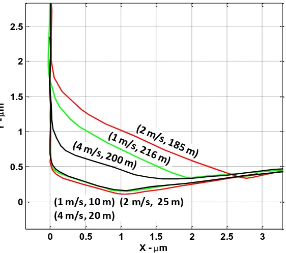
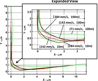
Figure 3-10. 2D wear areas for the orthogonal AISI1215 diamond turning tests a) low speed 2-8 mm/s, b) mid speed 71-284 mm/s, c) high speed 1-4 m/s. Note the vertical scale is different for each plot. ... 63

Figure 3-11: 100x zoom (70x50 μm window) SWLI surface measurement of AISI1215 surface. 122nm Ra, 165nm rms. ... 64

Figure 3-12: Arrhenius plot of mid and high-speed 2D wear area change vs. inverse of tool temperature determined from finite element models. ... 65

Figure 3-13: Arrhenius wear model and experimentally determined wear rates over 4 orders of magnitude of cutting speed. ... 66

Figure 3-14: Arrhenius wear model (Ea = 27.1 kJ/mol, A = 320 μm2/sec) for various depths of cut used in temperature formulation ... 67

Figure 3-15: Left: Stavax diamond turning experiment on ASG2500 DTM. Right: Magnified view of metal pickup on diamond rake face post-machining... 68

(14)

Figure 3-17: EBID worn tool cross-sections for diamond tool turning Stavax ... 70

Figure 3-18: Wear vs. machining distance for CT of Stavax ... 70

Figure 3-19: Arrhenius plot for diamond tool wear machining Stavax ... 71

Figure 3-20: Arrhenius wear model and wear data for Stavax compared to the Arrhenius wear model for AISI1215. ... 72

Figure 4-1: Plotted tool trajectories from equations of motion in tool and part coordinates ... 81

Figure 4-2: Critical timepoints evaluated on the ellipse in tool coordinates. ... 82

Figure 4-3: Critical timepoints evaluated on the ellipse in part coordinates ... 83

Figure 4-4: Spatial error as a percentage of ufpc produced by t1 and t2 estimation in Equation (4.12) ... 84

Figure 4-5: t1 and t2 timepoints evaluated in tool coordinates equations of motion ... 85

Figure 4-6: Example spatial error is 0.15% of ufpc from estimated t1 and t2 timepoints ... 86

Figure 4-7: Example timepoint calculations displayed in tool and part coordinates ... 87

Figure 4-8: Results from parametric study varying HSR. axb = 6x6 μm, DoC = 5 μm, f = 1 kHz, vwkpc = 0.063..3.98 mm/s. ... 92

Figure 4-9: Example 2D uncut chip shapes from parametric study varying HSR... 92

Figure 4-10: Results from parametric study varying ellipse shape. Ellipse swept area is kept constant (a*b = 16 μm2) and theoretical PV surface finish is constant according to equation (4.5). f=1 kHz, DoC = 5 μm , vwkpc = 0.081..14.608 mm/s (ascending left to right on graph). ... 93

Figure 4-11: Example 2D uncut chip shapes for varying ellipse ratios. ... 93

Figure 4-12: Results from parametric study varying horizontal amplitude, a. f = 1 kHz, vwkpc = 0.2 mm/s, DoC = 5 μm. Parameters not listed are constant. ... 94

Figure 4-13: Example 2D uncut chip shapes for varying horizontal ellipse amplitude, a. ... 94

(15)

Figure 5-2: Plastic strain rate and temperature contour plot results from 10kHz, 110x20 μm EVAM simulation. ... 105 Figure 5-3: Tool force and maximum temperature values of 10kHz, 110x20 μm simulation.

Timepoints a-d correspond to Figure 5-2. ... 106 Figure 5-4: Top: TecPlot plot of EVAM simulation data with high-order polynomial

interpolation. Bottom: Matlab plot of same data with 1000 point subsampling and 10 pt running average. ... 108 Figure 5-5: Example of cut force results from 10kHz, 110x20 μm simulation. Results are

shown after 1000-point subsampling and with different low-pass filtering via running average. ... 108 Figure 5-6: Left: Example of peak tool temperature in an EVAM simulation vs. time reaching

semi-steady state. Right: Expanded temperature profile of on EVAM steady state cycle highlighting contact and cooling zones. ... 109 Figure 5-7: Example integration of wear rate over contact time to determine average EVAM

wear rate. ... 110 Figure 5-8: Absolute EVAM parameters vs. relative EVAM parameters used to compare

calculated EVAM wear rates to the Arrhenius wear model ... 111 Figure 5-9. Relation of horizontal speed ratio to EVAM chip size ... 112 Figure 5-10: Thrust and cut force from FE EVAM simulations varying workpiece speed .... 114 Figure 5-11: Peak tool temperature from FE EVAM simulations varying workpiece speed 114 Figure 5-12: Comparison of average and peak EVAM tool temperatures vs. temperature rise

in conventional machining at workpiece velocity ... 115 Figure 5-13: Wear per time and wear per distance values for varying HSR. ... 116 Figure 5-14: Calculated 2D EVAM chip shapes using EVAMchip.m for simulations varying

(16)

Figure 5-18: Comparison of residual, average, and peak EVAM tool temperatures vs. temperature rise in conventional machining at workpiece velocity ... 122 Figure 5-19: Wear per time and wear per distance values for varying ellipse shape. ... 122 Figure 5-20: Forces from 1,4,10, and 40 kHz simulations. Top curves are cut force, lower

curves are thrust force. ... 125 Figure 5-21: Maximum tool temperatures for EVAM simulations varying frequency and

maintaining constant uncut chip shape and HSR ... 126 Figure 5-22: Temperature spike results of multi-frequency simulations vs. sliding distance. ... 127 Figure 5-23: Comparison of residual, average, and peak EVAM tool temperatures vs.

temperature rise in conventional machining at workpiece velocity. ... 127 Figure 5-24: Wear rate results for multi-frequency simulation set. ... 128 Figure 5-25: Calculated 2D EVAM chip shapes using EVAMchip.m for simulations increasing

frequency while reducing amplitude ... 130 Figure 5-26: Force results from EVAM simulations that frequency while reducing amplitude ... 131 Figure 5-27: Temperature spike results for EVAM simulations that simultaneously increase

frequency while decreasing amplitude. ... 131 Figure 5-28: Comparison of residual, average, and peak EVAM tool temperatures vs.

temperature rise in conventional machining at workpiece velocity. ... 132 Figure 5-29: Wear rate results for simulation set increasing frequency while decreasing

amplitude ... 133 Figure 5-30: Uncut 2D chip cross-sections for 110x20 μm and 55x10 μm simulations varying

frequency ... 134 Figure 5-31: Left: Average tool temperature rise vs. frequency for two ellipse sizes. Right:

Wear results for two different ellipse sizes ... 135 Figure 5-32: Wear / distance results for two EVAM simulation sets varying frequency

(17)

Figure 5-33: Wear / distance results for two EVAM simulation sets varying frequency calculated using relative EVAM parameters. ... 137 Figure 6-1. New flat+groove Ultramill toolholder design and kinematic linkage for elliptical

toolpaths ... 142 Figure 6-2: Front view of Y-axis tower and Ultramill setup ... 143 Figure 6-3: Side view of Ultramill experiment setup on the Nanoform ... 143 Figure 6-4: Left: Two-slot Ultramill toolholder design by Cerniway [52]. Right: New slot and

flat design removing kinematic over-constraint and increasing base thickness ... 144 Figure 6-5: Top Left: Pressure dial showing pressure vibration due to thermocube. Lower

Left: Pressure dial after fluid dampener installed. Left: Fluid dampener showing internal structure ... 145 Figure 6-6: Schematic of AISI 1215 steel fin workpiece, cutting orientation, and wear zones

on the tool for EVAM wear experiments varying frequency. ... 147 Figure 6-7: Tool forces measured during EVAM of AISI1215 steel at 1, 2, and 4 kHz. Forces

shown were acquired at approximately 100 mm cutting distance. ... 150 Figure 6-8. Conventional machining surface finish vs 1kHz EVAM surface finish on AISI 1215

steel. ... 151 Figure 6-9: EVAMed AISI1215 surface showed asperities approximately the same size as

alloy inclusions observed in polished surface of same material [129] ... 152 Figure 6-10. 2D worn tool cross sections for EVAM and conventional machining. ... 153 Figure 6-11: EVAM 1kHz EBID worn tool cross section compared to tools used in high and

low speed conventional machining. ... 154 Figure 6-12: 2D worn area calculated from EBID traces ... 155 Figure 6-13. Wear data from conventional machining of AISI1215 and EVAM tests varying

frequency compared to Arrhenius tool wear model. ... 156 Figure 6-14: Wear data from conventional machining of AISI1215 and EVAM using relative

(18)

Figure 6-16: Top: Cap gauge measurement results varying phase and voltage of Ultramill inputs. Bottom: Aspect ratio of measured ellipses varied with phase but not voltage similarly to Negishi’s measurements [105]. ... 161 Figure 6-17: Relationship between stack voltage and ellipse area. ... 162 Figure 6-18: Three toolpaths selected for multi-ellipse experiments confirmed via

capacitance probe measurement ... 163 Figure 6-19: 2D Uncut chip shape and resulting calculated parameters for three ellipse

shapes chosen for the multi-ellipse experiment. Units of EVAM parameters are in [mm] and/or [sec]. . ... 164 Figure 6-20: Tool forces for conventional machining of C360 brass at 2.53 mm/s. ... 166 Figure 6-21: Forces on workpiece measured during EVAM of C360 brass at 3 different

ellipse shapes and 2 depths of cut. ... 167 Figure 6-22: Zygo NewView SWLI surface measurement of AISI steel workpiece for three

ellipse shapes after 5m cutting distance. Cutting direction is right to left. ... 168 Figure 6-23: Surface traces made from of EVAMed steel surfaces in using different ellipse

shapes. ... 169 Figure 6-24: EBID cross-sections of worn tool edge after EVAM of AISI1215 using different

ellipse shapes ... 170 Figure 6-25 - Resulting wear from multi-ellipse test compared to wear model. Absolute

terms (workpiece speed and wear / machining distance, purple dashes) are compared to relative terms (wear / sliding distance and maximum horizontal tool tip velocity, blue diamonds) ... 171 Figure 6-26: Resulting wear from multi-ellipse test compared to wear model. Relative

terms use tangential velocity at maximum chip thickness as x-axis values (orange dashes). ... 172 Figure 6-27: Left: Son-X 80 kHz ultrasonic LVAM system. Right: Video monitor view of Son-X

(19)

Figure 6-28: AISI 1215 workpieces used in 80 kHz LVAM experiment (post machining). Workiece on the right has a protective cap installed ... 177 Figure 6-29: Test locations on two tools used to machine workpiece 1 and workpiece 2. 178 Figure 6-30: 50x zoom SWLI measurements (140x110 µm window) of AISI1215 parts

machined with Son-X ... 179 Figure 6-31: 100x zoom SWLI measurement (70x50 µm window) of workpiece 1 showed

vibration features at spatial frequency of 1192/mm or 0.839 µm... 180 Figure 6-32: 100x zoom, SWLI measurement (70x50 µm window) of workpiece 2 showed no

distinct vibration frequency. ... 180 Figure 6-33: EBID worn tool cross-sections of tools after 80 kHz machining AISI1215 fins. 181 Figure 6-34: Comparison of SonX 68 mm/s tool wear vs. mid speed conventional machining

tool ... 182 Figure 6-35: AISI1215 Son-X wear results vs. conventional machining wear model from

Chapter 3. Depth of cut for model and machining is 1 μm. ... 183 Figure 6-36: Top: Picture of two Stavax workpieces post machining. Bottom: Schematic of

different machining test areas. ... 187 Figure 6-37: Test locations on two round tools used for ultrasonic machining of Stavax ... 187 Figure 6-38: Projected 2D uncut chip areas for non-overlapping and overlapping cuts with

0.5 mm radius tool. ... 188 Figure 6-39: Talysurf profilometer tracing across Stavax Workpiece 1 ... 189 Figure 6-40: Talysurf profilometer trace of Stavax Part 1 (tests 1-3). ... 189 Figure 6-41: Zygo WLI surface measurement of Part 1 (Tests 1-3). For tests 2 and 3,

measurements are taken at the bottom of a groove and best-fit cylinder is removed. ... 191 Figure 6-42: Talysurf profilometer trace of Stavax Part 2 (Test 4-5) ... 192 Figure 6-43: Zygo SWLI surface measurements of test 5 grooves. Best-fit cylinder is

(20)

Figure 6-44: 100x SEM images of three wear zones on 80 kHz tool used to machine Stavax

... 194

Figure 6-45: EBID Traces of round tools cutting STAVAX ... 195

Figure 6-46: Comparison of Son-X tool after overlapping cuts on Stavax, and straight-edged tool high speed conventional cutting ... 195

Figure 6-47: Ultrasonic Stavax machining wear results (round tool) compared to conventional Stavax machining (flat tool). ... 197

Figure A-1: Skewed ellipse and uncut chip calculated using EVAMchip.m ... 221

Figure A-2: Vertical chip thickness calculated using EVAMchip.m ... 222

Figure A-3: Tangential tool tip velocity calculated using EVAMchip.m ... 222

Figure A-4: Example of selected pixels on an EBID line in digitize11 GUI ... 224

Figure A-5: Schematic showing wear area and worn surface measurements used to define ‘characteristic wear depth’ ... 225

Figure A-6: Description of ‘Worn Surface’ measurement used in definition of ‘Characteristic Wear depth’ ... 226

Figure A-7: Example of using EBIDautorot.m to align an EBID worn tool cross section ... 227

Figure B-1: Photograph through tabletop microscope showing metal pickup (Stavax 420 stainless steel) on the diamond cutting edge. ... 228

Figure B-2: Tool holders made for proper 45° tilting and placement in the JEOL6400 FESEM sample chamber... 229

Figure B-3: Preparation of diamond tool for EBID measurement with conductive carbon tape to reduce charging. ... 230

Figure B-4: Viewing port view in sample insertion chamber after setting tool and toolholder in the SEM stage dovetail mount. ... 231

Figure B-5: EBID stripe is made by scanning across the tool edge with initial tilt about X of 45° ... 232

(21)

(22)

L

IST OF

S

YMBOLS

 a, b – ellipse horizontal and vertical amplitude, respectfully (1/2 peak-to-valley width),.

 DoC – Depth of cut, distance from part surface to lowest point of ellipse

 ds – sliding distance per cycle, calculated section of tool trajectory which the tool is in contact with workpiece

 Ea– Activation energy

 f - EVAM frequency in cycles per second

 HSR – horizontal speed ratio, ratio of the workpiece velocity to the maximum tangential velocity of the ellipse.

 k – constant of proportionality between speed and tool temperature

 PVcross -theoretical PV surface finish in the cross-feed direction

 PVup. - theoretical PV surface finish in the upfeed (cutting) direction

 Ra– Arithmetic mean surface roughness

 rduty – duty cycle. The fraction of each vibration period which the tool is in contact with the workpiece.

 rup – sliding distance per upfeed ratio,ratio of ds to ufpc which can be multiplied by total cut distance to total sliding distance

 s – sliding distance

 ufpc – up-feed per cycle, the distance the center of the ellipse travels in one EVAM cycle.

 vmax_chip – tangential velocity at maximum chip thickness. Vector sum of tool tip velocity components evaluated at a location of maximum vertical chip thickness.

 vs – sliding speed of a tool against a workpiece. It can be used for VAM or conventional machining

(23)

 vx-max– maximum horizontal velocity. Maximum horizontal tool tip vibration velocity added to the workpiece velocity

 αmin– minimum tool clearance angle, equal to the angle of the tangent of the ellipse at the point where the tool enters the workpiece

 Δychip- maximum vertical chip thickness. Vertical thickness of the 2D uncut chip at the its maximum value

 σn – Normal stress

(24)

1 I

NTRODUCTION

1.1 D

IAMOND

T

URNING AND

T

OOL

W

EAR

The use of diamond as a cutting tool has a long history, with reported use going back to the 16th century for making finely spacing rulings and diffraction gratings. Use as a lathe tool for forming mirror-like surface finishes didn’t occur until the very early 20th century [1]. Diamond turning in its present form utilizes a single crystal natural or synthetic diamond as a tool to cut many different kinds of materials including metals, ceramics, glasses, and polymers. Single crystal diamond can be polished and formed to produce a very sharp and smooth cutting edge with edge radius often less than 20 nm and possibly less than 1 nm [2,3]. This smooth edge is reproduced on the cut or turned workpiece which allows optical quality surface finishes.

(25)

edge and precisely controlled machine motion enables optics to be made with sub-micron form error and optical quality surface finish (< 5 nm rms1).

Diamond turning currently finds use in a plethora of commercial, military, and research applications. DT allows an optical surface to be formed on a structural component itself, reducing the number of fabricated parts and manufacturing steps. An example of this is a scanner mirror in a laser printer, where reflective surfaces are machined directly onto the aluminum periphery of a spinning wheel. DT also allows some parts to be made without the need for finish polishing; for example, brass molds for contact lenses. Examples of other contemporary commercial applications include molds for phone camera lenses or master cylinders for rolling antireflective screens or lightguides for LCD displays. The most often cited military use for DT is in infrared (IR) optics. Brittle IR crystals like germanium (Ge), zinc selenide (ZnSe), zince sulfide (ZnS), or gallium arsenide (GaAs) can be diamond turned. Other brittle materials such as cadmium-telluride (CdTe) are used for high powered industrial C02 lasers [5]. Though this class of materials is very important to industry and research, the DT process for brittle materials is quite different than for ductile metals. Other than discussing research regarding tool wear after machining these materials, the focus of this dissertation is on ductile metals.

Though a relatively mature technology, application of diamond turning and precision machining is expanding to more and more applications and is increasingly becoming a competitive technology to lithographic methods for high-speed fabrication of 3D microstructure arrays [1]. Recent examples are the diamond micro chiseling (DMC) technique to form micro corner cube array retroreflectors [6], use of the nano fast-tool servo (nFTS) to form micro-scale diffractive patterns [7], or using single crystal diamond micro-tools formed by focused ion beam (FIB) to cut high aspect ratio 30 μm tall pillars [8].

1_{There is no standard for ‘optical quality’. This depends on the requirements of the specific optic and the}

(26)

The principle utility of diamond turning is the ability to create geometrically precise part form and surface finish. In the machining process, friction and contact of the diamond on the workiece will incur inevitable tool wear. This level of precision is contingent on tool wear, which may cause loss in part fidelity via one or more of the following:

1.) Increased form error due to recession of worn tool edge and/or increased “minimum depth of cut” [9].

2.) Part deformation as a result of high tool forces [10,11].

3.) Transition from ductile cutting to brittle fracture in turning brittle materials [12]. 4.) Subsurface damage or residual surface stress [13].

5.) Deterioration of surface finish due to spanzipfel formation [14].

(27)

The chemical wear of diamond and diamond tools has been a topic of scientific interest for decades. Cast iron scaifes have been used for over six centuries to polish diamond due to the increased polishing rate of the iron [20]. The known solubility of graphite in molten iron, nickel, or cobalt lead to the use of these metals as catalysts in the HPHT diamond synthesis process first developed by General Electric in 1955 [16]. The growth of diamond as an industrial cutting or grinding material in the 20th century brought further academic interest regarding chemical affinity between diamond and these materials and how it relates to tool wear. The 1970s initiated much research regarding diamond grain and tool wear when rubbing these chemical wearing materials [21,22,22-27]. There are two reasons this research has continued to today; a continued desire for ultra-precision fabrication of parts from chemically wearing material with processes that use diamond, and the still general misunderstanding of tool wear. This is reflected by Oomen and Eisses et. al. who noted that due to the complex nature of diamond tool wear, published results may not be comparable, and are sometimes contradictory [28].

(28)

sensors [31], they cannot be placed adequately close to the cutting zone without high risk of being damaged. Less difficult, but still challenging, is measuring diamond tool wear. Authors have accomplished this using scanning electron microscopy (SEM) [32-34], which has limited resolution due to charging of the insulating diamond by the electron beam in the SEM chamber. Others have used atomic force microscopy (AFM) [3,35,36], or used profilometer measurements of indentions made by pressing the worn diamond into softer metal [28,37-39]. In addition, many researchers simply use optical microscopy and/or compare one tool to another without a numerical value assigned. Wear patterns on a diamond may be sub-micron to 100s of microns in scale. The scale and form of diamond wear also varies between workpiece materials [32], therefore defining wear through a singular value becomes difficult. Authors have defined it by wear land length, edge recession length, surface area of the wear, volumetric tool material loss, and more. Chapter 2 gives a review of the different measurement methods and definitions of wear. Chapter 3 gives further review of past attempts to measure or model tool temperatures and a new to relate temperature and wear with a wear model.

(29)

Paul et. al. noted that VAM is likely the most economically feasible method for precision diamond machining of chemically wearing workpiece materials [19]2. Of each of the previous mentioned methods to combat tool wear, vibration assisted machining is the only one that has produced commercial accessories for use in a DTM, such as the El-50Σ elliptical vibration tool from Taga Electric Co. Ltd. or the Son-X 80 kHz LVAM from Fraunhofer IPT. Most research literature involving VAM and EVAM present the machining theory and technique, then give examples of the benefits via good surface finish and lower tool forces. These studies do not address the science behind the benefits, but rather present and extol improvements then provide conjecture regarding their sources. Though industrial application is growing with the commercial devices, the still misunderstood chemical wear process in conventional DT has hindered optimization of the VAM process, or clarified the reasons why it works.

1.2 VAM

R

ESEARCH AND

T

OOL

W

EAR

Research involving VAM in ultraprecision manufacturing has expanded since the seminal work in the early 90s by Shamoto and Moriwaki at Kobe University, Japan3. Their VAM research started with ultrasonic linear vibration assisted machining (LVAM, [49]), and later sub-ultrasonic elliptical-vibration assisted machining (EVAM, [50]) and has continued to today with ultrasonic EVAM [51]. The 1D LVAM process superimposes a linear vibration in the cutting direction, and the 2D EVAM proves uses and elliptical vibration shown in Figure 1-1. Research of ultra-precision machining using sub-ultrasonic or ultrasonic LVAM and EVAM currently include major contributors across the globe, specifically in Japan, Korea, Singapore, China, the United States, and Germany.

2

Paul et. al. did not mention workpiece surface plasma-nitriding [44-47]

3

(30)

Figure 1-1: Schematics of 1D linear vibration assisted machining (LVAM, left) and 2D elliptical vibration assisted machining (EVAM, right)[52].

(31)

VAM researchers who had hypothesized lower tool temperatures with VAM, but had not verified this experimentally or analytically. In summary, literature is very limited on DT temperatures, even more limited on transient DT temperatures, and the affect of VAM on tool temperature in general is not understood. Chapter 4 of this dissertation gives FEM results that concur with Babitsky’s higher VAM temperatures, but also shows that thermo-chemical wear can still be reduced under most conditions.

Wear measurement of diamond tools used in VAM is presented in multiple papers. Chapter 2 reviews many of these examples of wear measurements. Most of these papers present tool wear comparisons between conventional and VAM methods used to fabricate the same part. For many, this is limited to a side-by-side comparison of light-microscope images of the two tools. This provides a comparison, but does not show the true 3D nature of the worn tool or assign a numerical value to the wear. While comparisons can demonstrate the ability of VAM to reduce wear, it does not provide for a more in-depth analysis of how VAM produces a certain worn shape, the relationship between VAM wear and surface finish, or give a wear measurement value that states how much the VAM tool wears less than the conventional tool.

(32)

1.3 P

ROBLEM

S

TATEMENT AND

O

BJECTIVES

Though the benefits of VAM are well documented, the science behind the reduced wear and improved surface finish is not as thoroughly researched. A fundamental understanding of thermo-chemical diamond tool wear is missing as well, which is essential to understand VAM’s benefits. This research has two main objectives:

1.) Investigate diamond tool wear process for conventional DT of steel to provide a baseline understanding of the machining parameters that most affect this wear. 2.) Use this baseline understanding to predict and interpret (on a scientific basis) how

EVAM improves DT of ferrous alloys.

This dissertation approaches a more scientific understanding of diamond tool wear and VAM tool wear reduction through several methods uncommon or non-existent in literature:

1.) Wear modeling that incorporates temperature and wear measurements and describes diamond tool wear through a thermo-chemical mechanism.

2.) Finite element simulation of the EVAM process and tool temperature prediction. 3.) Quantitative measurement and comparison of wear after conventional diamond

turning and VAM.

(33)

2 B

ACKGROUND

In-depth knowledge of diamond tool wear suffers not from lack of study, but lack of comparable studies. This chapter describes the different techniques used to study diamond tool wear, including definitions, measurement methods, and factors that contribute to tool wear. In particular, thermo-chemical wear mechanisms are described. Literature sources studying diamond tool wear and macro-scale tool wear use different measurand definitions for wear. Certain wear characteristics are commonly used to describe cutting tool wear, and are presented here, though literature sources use a variety of measurement techniques to obtain numerical measurement of these characteristics. Diamond tool wear is typically sub-micrometer up to dozens of micrometers in scale and three-dimensional in shape, presenting challenge to measurement and inevitable measurement uncertainty. These challenges are presented in a wide array of techniques used to study and define diamond tool wear.

(34)

2.1 T

OOL

W

EAR

:

W

HAT IS MEASURED

?

W

HAT IS WEAR RATE

?

One hindrance to compare different diamond tool wear studies is the lack of an unambiguous definition of ‘wear’ and ‘wear rate’. Often, these terms are used in an indefinite manner. This is similar to the term ‘tool life’, ie. the Taylor tool life equation, which is only given tangible meaning when associated with an undesirable level of wear, surface finish, tool forces, form error, etc. To compare wear between experiments quantitatively, a numerical value needs to be assigned. Research authors define a measure of wear based on the measurement methods available. In addition, predictive modeling of wear requires a numerical value to relate to machining and material parameters and geometry.

Much tool wear research, including non-ultraprecision machining, measures tool wear by observing a feature in an optical microscope (often with Nomarski interference contrast) and noting a single length dimension, or simply comparing the observed level of wear between tests as ‘higher’ or ‘lower’ [19]. The true nature of diamond wear is three-dimensional and anything less than high-resolution 3D mapping of the worn surface requires geometric approximation or subjective comparison. Common wear patterns emerge which have yielded widely recognized and repeated definitions. These include one, two, and three-dimensional parameters. The following explains different definitions of measured wear and wear rates used in literature. ‘Wear rate’ is another often used term with multiple definitions depending on the author. Various measures of wear and definitions of wear rate are given in the following with literature examples and discussion of the limits of these measurands.

Wear land, width, edge radius, and crater wear:

(35)

a straight-edged tool. Varying depth of cut along the cutting edge due to cross-feed and a radiused tool promotes varying levels of wear.

If a worn tool cross-section (side view in Figure 2-1) can be obtained, fitting a circle to the edge to calculate edge radius is only valid if the radius of curvature is constant over a wide region. Varying radius of curvature will result in subjectivity errors dependant on the region chosen to fit.

Figure 2-1: Schematic of 1D cutting tool wear measures on a round tool.

Crater wear is more evident and detrimental to tool life in non-ultraprecision cutting and is the subject of multiple attempts to measure, model, and predict to optimize tool life [62-65]. It is less detrimental to diamond turning than wear land or edge radius. Oomen and Eisses measured crater depth of diamond tools by first observing in an SEM, then measuring with a Talystep profilometer and noted no correlation between crater depth and surface finish [28]. They also found that aluminum, electroless nickel, and copper resulted in different forms of crater wear that include a single wear groove or multiple perpendicular grooves. Though a single unit of measure is useful for comparison using the same

Edge Radius

Cut direction

Wear Land Crater

Wear Wear Width

Rake Face

W

e

ar

L

an

d

C

u

t d

ir

ec

ti

o

n

Clearance Face

Top

Front

Side

Cut direction (out of screen)

Rake Face

(36)

workpiece material, a different crater wear measurand is necessary to quantitatively compare between workpiece materials.

The wear land length may be especially difficult to define. The front of the wear land may be defined to begin at the rake face as depicted in Figure 2-1, or at the rake face minus the edge radius. The back side of the wear land may not have a distinct edge but may be rounded so that locating the end point is difficult. Brinksmeier et. al. made high resolution measurements of diamond tools using an atomic force microscope and used edge radius and wear land as measurands [35]. They did not clarify which portion of the tool was deemed the ‘wear land’. Arcona and Drescher simplified their diamond tool force models by only assuming and edge radius and wear land measurement and also assumed the wear land forms parallel to the cutting direction [10,11]. Nevertheless, it is been shown that the wear land may form at an angle to the cutting direction when diamond turning steel [32]. Wear measurements made in Chapter 3 of this dissertation also show that this angle varies with cutting speed on the same material.

Wear Area:

(37)

Figure 2-2: Schematic of different definitions of ‘wear area’ on a round tool.

Works by Wilks, Thornton, and Hitchiner et. al. use a simplified area [27,40,66,67]. Their wear area is approximated by multiplying the width of the wear, x, by the wear land length, y, shown in Figure 2-3, which overestimates the true value of the area. This simplification also neglect errors due to potentially dissimilar shapes of the wear between experiments, or the true three-dimensional nature of diamond tool wear.

1980

Figure 2-3: Schematic showing wear area defined by Thornton and Wilks [27,66].

Cut direction

Rake Face

C

u

t d

ir

ect

ion

Clearance Face

Cross-section worn area Flank

worn area Rake worn area Top

Front

Side Cut direction

(38)

Another example of measuring rake worn area projected from a viewing plane is made by Durazo-Cardenas et. al. shown in Figure 2-4 [12]. This is similar to the top view in Figure 2-2. In addition, they make wear width (WL) measurement and edge recession (dR).

Figure 2-4: Wear area defined by Durazo-Cardenas et. al. is area of edge recession along rake face [12].

Similar to the 1D measurands, 2D wear area measurements incur error based on geometric simplifications and neglecting wear patterns in out-of-plane directions. For example, the wear area defined by Thornton and Wilks in Figure 2-3 may neglect any convex curvature of the surface, which would yield a larger surface area than that projected onto their microscope viewing plane. The same goes for the rake worn area in Figure 2-1, though Durazo-Cardenas combined this area with other measurements to define the 3D shape of the tool.

Wear Volume:

(39)

Volumetric wear measurements in these static tests were aided by the relatively simple wear geometry. Diamond tool wear geometry, as previously mentioned, may be much more complex. Durazo-Cardenas et. al. estimated 3D tool wear volume using geometric approximations based on Talysurf measurements of plunge cut grooves combined with direct observation of tool wear via SEM [12]. They used definitions of maximum edge recession and wear width to calculate calculate the wear volume. This calculation assumed the wear land was parallel to the cutting direction.

The 2D worn area exhibited on the side view in Figure 2-2 is easier to relate to wear volume and is more practical for wear modeling purposes. Most ultra-precision cutting can be assumed a plane-strain, 2D process that occurs in this 2D plane as long as the contact width is much greater than the depth of cut. If the wear is constant along the tool edge, then the wear volume can be approximated as this 2D wear area multiplied by the out of plane width. This idea is utilized by the wear measurement method used in this dissertation described in Chapter 2 Section 1.2, and wear experiments conducted in Chapter 3 and 6.

Wear rate:

The term ‘wear rate’ is used often in literature, but refers to different units of measurement. Rates assume one of the aforementioned 1D, 2D or volumetric measures per unit time or distance. Distinction between time or distance rate definitions is important, since these rates may be a function of velocity. For example, the wear/time may be high for a high speed machining experiment. Due to the high speed the distance cut will be very large, therefore the wear/distance may be small. This is discussed further in the development of the wear model of Chapter 3.

(40)

probability of a wear asperity forming and contributing to the wear volume. Takeyama and Murata defined non-ultraprecision tool wear rate as volume per contact area per time, yielding a length per time units similar to the static diamond wear tests [71]. This is more directly relatable to a 1-D diffusion approximation for the wear mechanism, but inaccurate volume and area measurements at the micro-scale impede its use. Similarly, Paul and Evans et. al. defined wear as a reaction rate defined as number of atoms or moles per contact area per time in their chemical wear analysis [19]. Their experiments did not present measured values for carbon atoms lost from the diamond due to wear, but provided relative comparisons between observed wear.

Works by Wilks, Thornton, and Hitchiner et. al. define wear rate as their wear area shown in Figure 2-3 per unit of machined surface area [27,40,66,67]. This is similar to a 1D wear per distance rate, as the width of their wear is of the same order as the tool contact width, thus cancelling in the numerator and denominator and leaving cut distance in the denominator.

Definition of time or distance wear rate is complicated by the VAM process. An EVAM tool contacts the workpiece and chip over a longer distance than the actual machined length. Also, an EVAM tool contacts the workpiece over a shorter time than the total machining time. These unique terms for EVAM time and distance are defined in Chapter 4. Special consideration of these terms are used when comparing EVAM tool wear results in Chapter 6 to the wear model in Chapter 3, and finite element models in Chapter 5.

2.1.1 DIAMOND TOOL WEAR MEASUREMENT TECHNIQUES

(41)

given in Figure 2-5. These optical microscope images can be related to the wear length and area definitions in Figure 2-1 and Figure 2-2. Brinksmeier et. al. used optical microscope images to measure wear land [73]. Most authors only provide the subjective comparison.

Figure 2-5: Microphotograph of rake face and flank face of round diamond tool from [72]. ‘Upper boundary’ indicates region nearer the feed direction.

Optical microscopy has two limitations: resolution and depth of field is limited and inferior to other microscopic methods (AFM or SEM) and resulting image only offers 2D measurement.

2.1.1.1 ATOMIC FORCE MICROSCOPE (AFM) DIRECT MEASUREMENT

Multiple authors have used atomic force microscope (AFM) measurements to describe tool wear [2,3,35-37,44,73]. Gao et. al. noted the difficulty in aligning a diamond edge with the AFM probe tip, so they developed a procedure to align both the diamond and probe tip at the focal point of a diode laser [36].

(42)

full 3D characterization of tool wear, but does suffer from some technical issues. Apart from tool edge and probe tip alignment issues, the AFM probe tip can become damaged or worn resulting in unknown tip geometry. Periodic measurement of a reference artifact may be necessary.

2.1.1.2 INDENTATION/SURFACE MEASUREMENT

Another method used is to indent a worn tool into a soft metal workpiece, or make small grooves that replicate the worn edge. These indentions or grooves can then be measured. The major detriment and source of error for this method is the material springback, or elastic-recovery in the indented material. One great benefit of this method is that it can be easily incorporated into a machine setup. Indention material may be placed in the machine workpace and indented after successive wearing cuts. This method is limited to small levels of wear, however. As wear characteristics (wear land, edge radius, etc.) increase in scale, they require deeper grooves or indentions. This, in return, incurs more potential error from material springback.

(43)

2.1.1.3 SCANNING ELECTRON MICROSCOPE (SEM)DIRECT MEASUREMENT TECHNIQUES

The majority of diamond tool wear researchers use direct observation of a diamond edge in a scanning electron microscope (SEM). The result is similar to using an optical microscope, but with image zoom values more than 50,000x and a possible depth of field and order of magnitude greater than the field of view. Two main problems occur when viewing a diamond in an SEM. The first problem is the same as for optical microscopic images, namely trying to characterize a truly 3D shape with a 2D method. Secondly, diamond is an insulator4, which results in electric charging from the electron beam. This inhibits secondary electrons to escape from the sample surface, and requires low accelerating voltage (<4 kV) until the incoming beam current can equal the outgoing secondary and backscattered electron current. This limits the imaging resolution, and features less than 50 nm are difficult to discern.

Some wear measurements can be made with alignment of the tool with the focal plane to measure length or area wear parameters described in Figure 2-1 o Figure 2-2. Durazo-Cardenas et. al. used this technique to make wear land measurements to compare with their tool imprint measurements [12]. Malz et. al. also made wear land measurements and from SEM images to compare to AFM results [44]. Casey and Wilks explored using different measureands such as wear width, edge recession, and wear land length [74]. They decided edge recession was best due to ease of alignment within the SEM, and the edge recession increased linearly with work distance.

Asai et. al. overcame the 2D image problem by using two secondary electron detectors in an SEM [75]. In their method, a focused electron beam is scanned perpendicular to the cutting edge. A computer then determined the angle of inclination of the reflecting point, which is integrated to form the tool edge profile. This creates a cross-section of the tool edge, and

4_{This is with the exception of ‘blue’ diamond with boron impurities that make it a semi-conductor, or}

(44)

multiple cross-sections could be made to form a 3D map of the wear surface. This method requires specialized equipment not common in most SEMs.

Yet another technique to distinguish a semi-3D wear shape from 2D SEM images is to use a contrasting agent via electron-beam induced deposition (EBID) [33,34]. This technique ‘paints’ a line of hydrocarbon contamination over the worn tool edge by line scanning the electron beam in the SEM. The basic concept is outlined in the following section, and directions for obtaining EBID tool wear measurements used in this dissertation are described in Appendix B.

2.1.2 ELECTRON BEAM INDUCED DEPOSITION (EBID)TOOL WEAR MEASUREMENT METHOD

The electron beam induced deposition method (EBID) was developed by J. Drescher at NC State University as part of his Ph.D. thesis [10]. While observing diamond tools at low accelerating voltage as to reduce charging, he noticed 3D topographical information was difficult to discern from the relatively smooth and featureless tool edge. Concurrent research at NC State was using hydrocarbon contamination growth in an SEM to create AFM probe tips [76]. The contamination growth technique was taught to Drescher, who used the contamination growth as a contrasting agent to distinguish the tool edge in his SEM measurements. Use of the EBID method has been limited to researchers at the Precision Engineering Center at NC State, but has been used in multiple papers, theses, and dissertations studying diamond tool wear [10,11,32-34,77,78].

(45)

stretched SEM image is compared against the included angle of the actual tool (90o – clearance angle). The vertical image size is then readjusted until the image included angle is within 1o of the real tool included angle. The code then changes the scale of the image from pixels to microns according to the SEM image measurebar, and rotates the cross-section to align with other collected cross-sections for direct comparison. Worn cross-section area is determined by calculating the area enclosed by the EBID stripe and two best-fit lines that run along the EBID stripe where it contacts unworn clearance and rake faces. Worn tool cross-sections made from EBID images are rotated and aligned so that the original tool point exists at the origin of the plot. Lines corresponding to the rake face of the tool align with the y-axis.

Figure 2-6. Top Left: Viewing angle of EBID stripe on the diamond edge. Top Right: Example EBID image. Bottom: Worn area and cross-section measurement via Matlab script. SEM View

Diamond Rake Face

Carbide Insert

1 m

EBID Stripe

8 points create clearance face

8 points create rake face Interpolated line

(clearance)

Worn area between interpolated lines

and EBID stripe Interpolated line _(rake)

SEM View

Diamond Rake Face

Carbide Insert

1 m

EBID Stripe

8 points create clearance face

8 points create rake face Interpolated line

(clearance)

Worn area between interpolated lines

(46)

2.2 F

ACTORS

A

FFECTING

D

IAMOND

T

OOL

W

EAR

In non-ultraprecision machining, the term ‘tool life’ has been described by Taylor’s equation since the early 1900s to describe the time period before a certain unacceptable level of surface finish, cutting forces, or other factor related to tool wear (ASTM B94.55M, 1985). Generally, metals deemed ‘diamond turnable’ can achieve tool life or machining distances on the order of 10s to 100s of kilometers before needing to be replaced [28,79]. These include, but aren’t limited to copper, brass, aluminum, and phosphorized nickel. Other important engineering materials that are not diamond turnable include iron, tungsten, or titanium alloys [19].

Good surface finish and form accuracy is the principle goal of diamond turning. Peak-to-valley surface finish is often estimated through purely geometric considerations based on the tool nose radius and feed via the formula PV=f2/8R. This formula is quite accurate for smaller tool radii and low levels of wear, but higher PV values result with tool wear [79]. This has been attributed to formation of spanzipfel, or elastic material springback at the intersection of neighboring tool passes [14]. This is also called plastic side flow by some authors [80]. Equation Chapter 2 Section 1

(47)

dislocation density is related to residual stress on the workpiece surface, which is also exacerbated by tool wear [13]. Ultraprecision VAM researchers have shown that the MTC may effectively by reduced with VAM and is decreased further with higher frequencies and lower vibration amplitude [84].

Tool forces also increase with tool wear. Typically, cut force (directed in the cutting direction) increases slightly with wear, while thrust force (directed out of the workpiece) increases at a faster rate [79]. It is been shown that thrust force increases and eventually surpasses cut force as the tool wears due to the increasing contact between the tool wear land and workpiece [10]. Drescher, and later Arcona also developed tool force models based on their experimental observations that considered worn tool geometry [10,11,78]. These were developed for use as predictive models to determine the state of tool wear before surface finish degraded to an undesirable level. There have also been successes in measuring acoustic emission and correlating changes in signal to deteriorating surface finish [85-87].

Multiple factors have been attributed to diamond tool wear. The following gives a background of some of the known contributors. Special attention is given to factors that contribute to thermo-chemical wear on non-diamond turnable materials.

2.2.1 ABRASIVE WEAR

(48)

that low-carbon steel of comparable hardness exhibited a similar level of wear at 1000x shorter distance and produced far inferior surface finish. Crompton, Hirst, and Howse also used the Archard wear coefficient, normalized with workpiece material hardness, in their rubbing experiments [23]. They also noted higher diamond wear rates when rubbing oxidized aluminum surfaces compared to clean surfaces. They attributed this higher rate to the harder almuminum-oxide surface causing increased abrasive wear.

2.2.2 WORKPIECE CHEMISTRY

Paul and Evans et. al. gave a thorough treatise on the chemical aspect of diamond tool wear in their 1996 Precision Engineering paper [19]. The focus of the paper was the correlation between materials that exhibited high levels of chemical wear, and the number of unpaired d-shell electrons in the constituent workpiece elements. Miyoshi and Buckley noticed a similar relationship with unpaired d-shell electrons and the friction of single crystal diamond (SCD) sliding on transition metals [88], though this work was not mentioned by Paul and Evans. In addition to the d-electron correlation, Paul and Evans gave a thorough treatise and review regarding the possible reactions involved in chemical diamond tool wear.

Paul and Evans et. al. surmised that carbon atoms from the diamond lattice would form intermediary chemical complexes with the workpiece material. Once the complexes are formed, the carbon may follow several pathways simultaneously and at different rates: return to the diamond crystal lattice, convert to graphite, react with other materials present, or diffuse into the chip or workpiece. They also noted that each of these individual processes are governed by the Arrhenius function, but with varying dependence on thermal energy energy barrier, or activation energy. The Arrhenius equation is:

exp Ea

k A

RT

  

 _ _

(49)

where k is the reaction rate constant, A is the pre-exponential constant with same units as k, Ea is activation energy, R is universal gas constant (8.314 J/mol/K), and T is temperature in degrees Kelvin. The units of k and A depend on the order of reaction; a chemical kinetics concept where order depends on the number of reactants and type of reaction [89]. The same equation defines temperature-dependence on the diffusivity constant in Fick’s laws of diffusion [90].

(50)

and inability of a concentration gradient to form in the workpiece. Jiang’s work is detailed further in Chapter 3 in discussion formulation of a chemical wear model.

Noting the relationship between tool wear and chemistry, researchers have attempted to vary surface chemistry of a workpiece to reduce wear. One of the more commonly diamond turned metals, electroless nickel, is a plated form of nickel with significant amount of phosphorous content (>10%), making it chemically inert to diamond. Pure nickel itself causes catastrophic chemical tool wear. Electroless nickel’s popularity as a DT material is reflected by the depth of understanding regarding tool wear behavior vs. phosphorous content and annealing temperature [26,39,95,96].

Malz and Brinksmeier et. al. investigated multiple hard nitride coatings, with the most successful results from titanium nitride [44]. Later, Brinksmeier et. al. incorporated nitride layer on iron [47]. They noted that while tool wear was minimized, the hard coating caused high machining forces which produced vibrations and reduced surface integrity. Chao et. al. was able to obtain surface finish better than 3 nm Ra by plasma nitriding the surface of stainless steel before diamond turning [45]. Wang et. al. continued this idea and machined a Fresnel optic out of AISI4140 die steel that was plasma nitride. On a test flat machined before the Fresnel optic, they obtained a surface roughness below 20 nm rms up to a machining distance of 5.4 km.

2.2.3 ATMOSPHERIC PRESSURE (OR AVAILABILITY OF OXYGEN)

(51)

Figure 2-7: Wear rate (wear area / machined surface area in 10-6 mm2/mm2) of single crystal diamond tool as a function of air pressure at cutting speed of 0.013 mm/s (left) and 0.13

mm/s (right) [27]. Curve and transition range are added for clarity.

At higher cutting speeds (1-11 m/s), Thornton and Wilks noted a wear value of 10 (10-6 mm2/mm2) that varied little with speed. When subjected to vacuum, the wear rate dropped approximately 50%, but had less affect at higher speeds up to 30 m/s.

Paul and Evans et. al. related the findings of Thornton and Wilks to their chemical wear analysis [19]. They surmised that at conventional DT speeds (1-11 m/s), wear proceeded by the formation of a metal-carbon-oxygen complex and is somewhat affected by the availability of oxygen. At high speeds (>11 m/s), high temperature allows metal-carbon complex formation (graphitization) which dominates the wear and the availability of oxygen plays no role. At low speeds (<0.13 m/s), their reasoning was a bit unclear from the text. Paul and Evans claim that high pressure and low speeds allowed other gaseous species to penetrate the workpiece, thus retarding the catalytic reaction with oxygen. Lowering the pressure allowed only oxygen to be available, thus catalyzing and causing a higher reaction rate.

VAM likely allows air or cutting fluid to enter between the tool and chip from the periodic tool-work separation. Based on the hypothesis that oxygen contributes to chemical wear, it would seem that dry VAM would increase the availability of atmospheric oxygen in the

Material Effects and Tool Wear in Vibration Assisted Machining.

ABSTRACT

BIOGRAPHY

ACKNOWLEDGMENTS

TABLE

OF

CONTENTS

L

IST OF

T

ABLES

L

IST OF

F

IGURES

L

IST OF

S

YMBOLS

1

I

NTRODUCTION

1.1

D

T

T

W

1.2

VAM

R

T

W

1.3

P

S

O

2

B

ACKGROUND

2.1

T

W

:

W

?

W

?

Rake Face

Clearance Face

Rake Face

Rake Face

Clearance Face

2.2

F

A

D

T

W