FMS loading with reliability consideration.

(1)

University of Windsor University of Windsor

Scholarship at UWindsor

Electronic Theses and Dissertations Theses, Dissertations, and Major Papers

1-1-1995

FMS loading with reliability consideration.

Abi M. Philipose

University of Windsor

Follow this and additional works at: https://scholar.uwindsor.ca/etd

Recommended Citation Recommended Citation

Philipose, Abi M., "FMS loading with reliability consideration." (1995). Electronic Theses and Dissertations. 6744.

https://scholar.uwindsor.ca/etd/6744

(2)

FMS LOADING WITH RELIABILITY

CONSIDERATION

By

Abi M. Philipose

A thesis subm itted to the

Faculty o f Graduate Studies and Research through the Department o f Industrial and M anufacturing System s Engineering in partial fulfilm ent o f the requirements fo r

the Degree o f M aster o fA p p lied Science a t the University o f Windsor

UNIVERSITY OF WINDSOR

W indsor, O ntario, C anada

(3)

UMI Number: EC55039

INFORMATION TO USERS

The quality of this reproduction is dependent upon the quality of the copy

submitted. Broken or indistinct print, colored or poor quality illustrations

and photographs, print bleed-through, substandard margins, and improper

alignment can adversely affect reproduction.

In the unlikely event that the author did not send a complete manuscript

and there are missing pages, these will be noted. Also, if unauthorized

copyright material had to be removed, a note will indicate the deletion.

ProQuest LLC

789 East Eisenhower Parkway P.O. Box 1346

(4)

(5)

To

God

(6)

I hereby declare that I am the sole author of this thesis. I authorize the

University of Windsor to lend this thesis to other institutions or individuals for the

purpose of scholarly research.

Abi M. Philipose

I further authorize the University of Windsor to reproduce this thesis by

photocopying or by other means, in total or in part, at the request of other institutions

or individuals for the purpose of scholarly research.

(7)

The University of Windsor requires the signatures o f all persons using

(8)

ABSTRACT

Availability, flexibility, an d productivity are the m ajo r reasons luring

m anufacturers to o p t for Flexible M anufacturing Systems (FM Ss). Experience

has show n th a t the equipm ent and hardw are alone does n o t get the production

facility to this goal. Scheduling and production planning, especially loading,

plays a n im portant role in determ ining the efficiency o f the production facility.

T his research deals with loading a F M S, with reliability considerations.

It is desirable to ru n a production plant at 100% reliability. However, the

costs involved in increasing the reliability varies in a non-linear trend. Realising

the im portance o f the reliability facto r in production planning, three

m athem atical m odels were developed. Tw o o f the m odels were full loading

problem s, while the third is a partial loading problem . W ith the objective o f

m inim izing the tooling costs, the larger m odels p artitio n the dem and into

batches, assign batches to machines, assign tools to machines, and determine the

location o f the spare tools. The smaller m odel assumes th a t the batches are

assigned to m achines, by other m eans, and so this m odel assigns tools to

m achines an d determines optim al spares. A lthough newer an d true F M S have

tool sharing capability, the older systems do not. M athem atical m odels were

developed for b o th these cases.

F o r the first time, the reliability factor has been coupled directly w ith the

m athem atical loading m odel. H ypothetical, b u t realistic problem s have been

(9)

ACKNOWLEDGMENTS

I would like to express my appreciation to my supervisor Dr. S.M. Taboun, for

his advice, criticism, patience, and moral support during the course of this research.

I would like to thank to my committee members, Dr. M. Ahmadi and Dr. M. Wang, for

their time and advice.

I would like to thank Mr. Tom Williams, computer system manager, and Ms.

Jacquie Mummery, secretary of the Industrial and Manufacturing Systems Engineering,

for their help and assistance.

I wish to express my gratitude to all my friends, especially V.K. Damodran,

S.R.V. Majety, Alper Ozdemir and A. Atmani for their support, stimulating discussions

and friendship.

I would like to thank my parents for their love, support and encouragement

during the entire period of my education.

Finally, I thank my wife and children, who patiently endured difficult times, and

(10)

LIST OF TABLES

Table 2.1 Statistical Distributions useful in Reliability Engineering 12

Table 5.1 Process Plans and Processing Times, Model 1 Case 1 65

Table 5.2 Machine Capacities, Model 1 Case 1 65

Table 5.3 Tool Life and Tool Cost, Model 1 Case 1 66

Table 5.4 Dividing Demand into Batches and Assigning to Machines, M1C1 66

Table 5.5 Assigning Tools and Spares to Machines Model 1 Case 2 66

Table 5.6 Dividing Demand into Batches and Assigning to Machines M1C2 68

Table 5.7 Assigning Tools and Spares to Machines, Model 1 Case 2 69

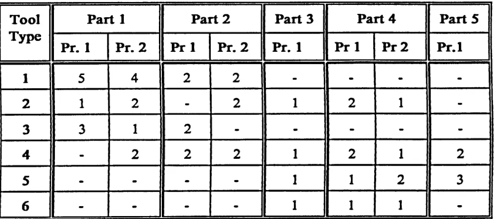
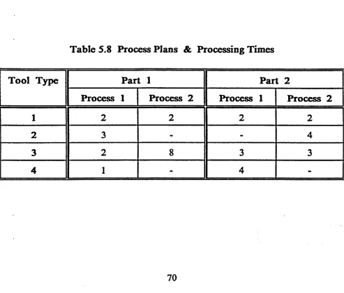
Table 5.8 Process Plans and Processing Times, Model 2 Case 1 70

Table 5.9 Machine Capacities, Model 2 Case 1 71

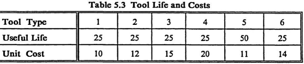
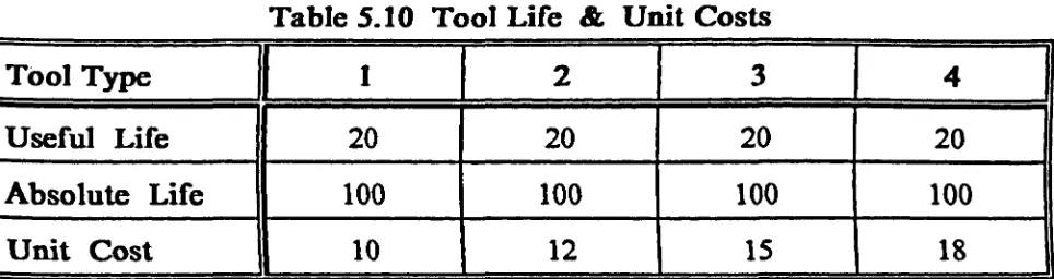
Table 5.10 Tool Life and Tool Costs Model 2 Case 1 71

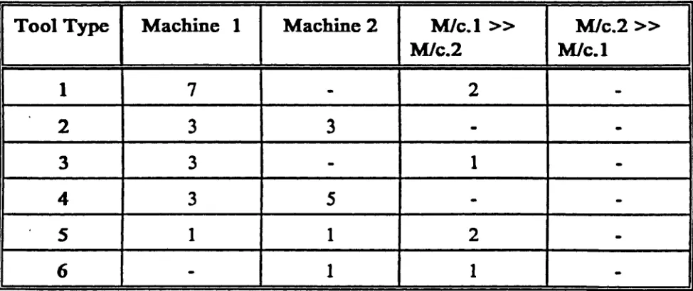
Table 5.11 Assigning Tools and Spares to Machines Model 2, Case 1 71

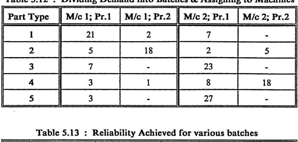
Table 5.12 Dividing Demand into Batches & Assigning to Machines 73

Table 5.13 Reliability Achieved for Various Batches 73

Table 5.14 Cycle Times of Operations in the System, Model 3 Case 1 76

Table 5.15 Effect of Required Reliability, on Total Cost and

Magazine Occupancy, Model 3, Case 1 77

Table 5.16 Redundancies used v/s Required Reliability, for Machine 1 80

Table 5.21 Effect of Required Reliability, on Total Cost and

(14)

Table 5.22 Redundancies used v/s Required Reliability 86

Table 5.23 Magazine Occupancy and Total Cost, Compared to Case 1 87

Table 5.24 Cycle Times for Operations in the System,

for Simulation Analysis 92

Table 5.25 Useful Tool life of Tools in the System 92

Table 5.26 Demand Partitioned into Batches, by the Mathematical Model 92

Table 5.27 Spares Used for Deterministic Cycle Times, Case 1 93

Table 5.28 Spares Used for Stochastic Cycle Times, Case 1 93

Table 5.29 Spares Used for Stochastic Cycle Times with

Catastrophic Failures, Case 1 93

Table 5.27 Spares Used for Deterministic Cycle Times, Case 2 95

Table 5.28 Spares Used for Stochastic Cycle Times, Case 2 95

Table 5.29 Spares Used for Stochastic Cycle Times with

Catastrophic Failures, Case 2 95

(15)

LIST OF FIG URES

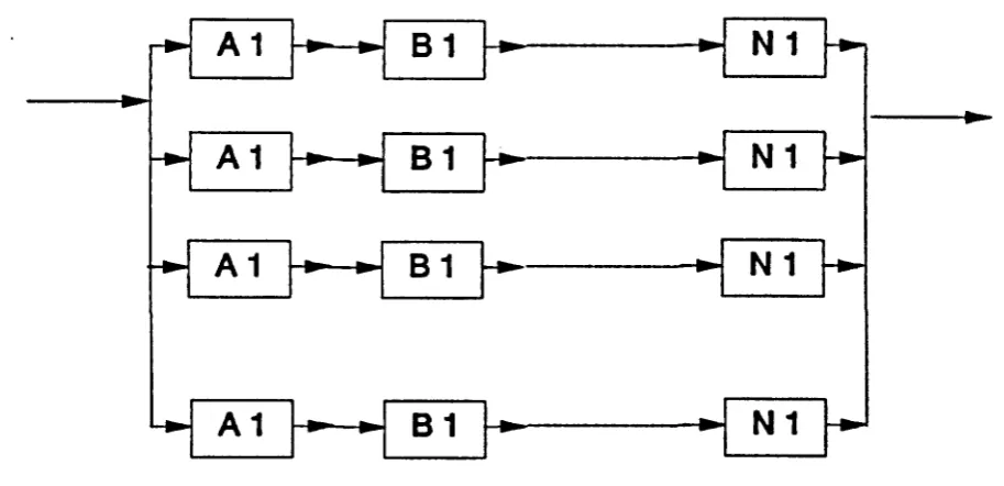
Figure 2.1 Representation of a Series System 13

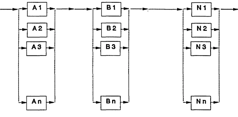
Figure 2.2 Representation of a Parallel System 13

Figure 2.3 Standby Redundancy, with Switching Device 14

Figure 2.4 Representation of a Series System with Standby Redundancies 14

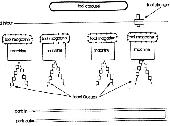
Figure 4.1 Typical Configuration of the System Being Studied 42

Figure 5.1 Effect of Reliability on the Total Cost 78

(16)

CHAPTER 1 INTRODUCTION

1.1 An Overview

Since the turn o f the century, the markets of the world are progressively

integrating into one global market. At the same time, the market has been steadily

drifting from a seller’s market to a buyer’s market. In the earlier days of the century,

a flourishing businessman stated, ’’people can order any colour of car as long as it is

black’’. Today, the company offers hundreds of colour and shade combinations for its

customers to choose. Besides variety, it is important to treat time as a critical source of

competitive advantage. So, trimming manufacturing lead time and product

development time are also of great importance. Thus, the changing market trend

demands efficiency, quality, flexibility and ingenuity from the manufacturers.

To compete in such a global economy, flexible manufacturing systems has

(17)

Flexible manufacturing has the potential to achieve the productivity of mass

production, while still offering a wide range o f flexibility. A Flexible Manufacturing

System (FMS) can be defined as a set of CNC machines and supporting workstations

that are interconnected by an automated material handling system and controlled by

a central computer (Askin 1993). Reduced labour, improved machine utilization,

improved operational control, improved product quality, reduced floor space

requirement and reduced inventory are some other benefits of using FMS.

Although FMS provides significant economic production in the long run, such

systems are highly capital intensive. Financial justification forms an integral part of an

FMS implementation. While too much or too soon creates excessive work in progress,

too little or too late leads to under-utilization of the facility. To maximize the return of

investment, one has to use the facility optimally. Flexible manufacturing being different

and similar to conventional manufacturing systems, it provides new and extensions of

older problems of operation research. The problems include designing the required

system, planning the operation to maximize the plant utilization, carrying sufficient

redundancies like tools, for an uninterrupted operation, and scheduling for the

production period. A high degree of system reliability is imperative in the operation of

(18)

In setting up an FMS, two groups of problems have to be addressed - Design and

Operational. The Operational problems can be further sub-divided into Planning,

Scheduling, and Control problems -(Stecke 1983). This research focuses on the loading

o f the FMS, which is a part of the planning sub-section o f the operational problem.

When FMS is employed for machining, assembly, or fabrication, they use a set

of tooling to perform the function. The system calls these tools sequentially, to perform

the desired operations. The tools wear out, break, or require resetting and maintenance,

from time to time, during the production run. Industrial data indicate that tooling

accounts for 25-30% of the fixed and variable cost of production in an automated

machining environment (Ayres 1988). Shaw (1980) described tool breakage as the

single most significant factor that reduces the productivity of manufacturing systems.

A key requirement for an efficient operation of an FMS is the existence of a

comprehensive tool management system. A certain level of reliability is required o f the

individual tools and the tooling system as a whole to ensure an uninterrupted,

production run. Sufficient redundancies must be foreseen at the preliminary production

planning stage, to cope with the various tool requirements. Whereas the cost of

redundancy is a negative factor, the additional reliability gained is a positive factor. So,

(19)

1.2 Objectives o f the Research

The objective o f this research is to develop a model for loading an FMS.

Machine Loading is defined as the decision associated with allocating jobs and the

required tools among the machining centres, subject to restrictions on the system. The

machine loading problem includes three entities; viz, the job, the tool and the machine.

A model taking care of all three entities would be a full machine loading model.

Otherwise, the problem is called a partial loading problem.

Flexible manufacturing systems in their complete form will allow tool sharing

between machines, via a gantry or monorail robot arm. However, tool sharing would

need additional investments in terms of equipment required, and more complicated tool

management policies. In practice, there are many FMS systems, where tool sharing is

not possible.

In this research, three sets of models have been considered. Each model is

formulated for two conditions. One, where tool sharing is permitted, and the other,

where tool sharing is restricted.

(20)

demand o f parts to be processed, process plans available to process the parts, number

o f machines available for the production period, the span of the production period,

capacities o f the tool magazines, and tool types available, the formulation divides the

demand into optimal batches, assigns process plans to the individual batches, assigns

batches to machines, assigns tool types to machines, determines their optimal spares

level, and the locates the spares in the different magazines. The objective is to minimize

the tooling costs.

A manufacturer always desires 100% reliability from the production shop.

However, higher reliability also costs more. The second model considers all the loading

problems and constraints mentioned above and then minimizes the tooling cost, and

also calculates the reliability with which an optimal batch is being processed by the

facility.

In many practical cases, the parts may not be assigned to the machines, based on

the similarity of their operations alone. In such cases, the demand will be partitioned

into batches and assigned to be processed by a particular process plan. Whereas the

second model made an evaluation of the reliability of processing a batch, this model

provides a generic solution to assigning tool types to machines, and optimizes the

(21)

minimum specified reliability. A linear program was developed that accommodated the

non linear reliability requirement.

Numerical problems were solved using the formulated models to test their

validity. The problems and their solutions have been provided.

Organization o f the Research :

The documentation of the research is organized as follows. A literature review

o f the past research works on tool life, tool life management, loading problems and

solutions in automated manufacturing, and analogous research is presented in Chapter

2. Some basic and important definitions, concepts and mathematics have been reviewed

in Chapter 3. Chapter 4 introduces the definition of the loading problem being

considered in this research. Nomenclature used have been shown. Later the three

models, each with two case scenarios have been derived. In Chapter 5, hypothetical, but

realistic numerical problems were taken up and solved using the derived mathematical

models. Some o f the results obtained were verified using a simulation model using

Witness simulation package. Conclusions and recommendations for future work have

been presented in Chapter 6. Various formulations done on Lindo, Lingo, Witness, and

(22)

CHAPTER 2 TERMS AND DEFINITIONS

Before taking up an FMS loading problem, with reliability considerations, and

building mathematical models, it would be advantageous to review some fundamental

concepts and definitions. A flexible m anufacturing system can be defined as an

arrangement of CNC machines, interconnected by an automated material handling

system, where the processing and movements o f the workpiece is controlled in

conjunction with a central computer. An FMS thus has the advantage of having the

capability to process a wide variety of products, in a near random order. One can now

visualize that the critical factor determining the performance of an F M S is ensuring the

optimal availability of machines and tools, as the demand for a certain workpiece comes

up, in a random order.

It is thus important to concentrate on the operational problems to achieve an

efficient operation. Loading is the focal point of production planning. Loading an

(23)

their attributes, and assigning the available machines and tools to process the demand.

Therefore there have been numerous research studies, dealing with loading an FMS.

Tool m anagem ent is the capability of having the required tools on the

appropriate machines, at the right time, so that the desired quantities of workpieces are

manufactured, while maintaining acceptable utilization of assets (Tomek 1986).

Gaalman (1987) described to o l sharing as a situation where the unavailable tool on a

machining centre, at a particular time, can be borrowed from other machining centres

in the system. Although a modem FMS would have tool sharing between machines,

there are older and lower capital systems where this facility does not exist. In this

research, both these scenarios were studied and modelled separately, and the numerical

results compared.

R eliability can be defined as, "the probability that an item (or system) will

perform its function adequately for the desired period of time when operated according

to the specified conditions." (Dhillon 1982). In other words, reliability is concerned with

determining the probability that a system consisting of many components will perform

its function. A system, where all constituent parts must function successfully, in order

to get a complete system performance is called a series system. Thus, in a system of this

(24)

at least one of the similar constituent parts has to function well for the system to

perform is called a parallel system. Schematic representation of a series and parallel

systems have been shown in Figure 2.1 and Figure 2.2.

Achieving higher reliability level often leads to the use of functional elements

that are interchangeable modular components, or redundancies. Redundancy could be

system level, or state level. System level of redundancy, also called high level

redundancy, often means higher capital costs and lower utilization levels. State level,

or component level is a more popular redundancy strategy. The state level redundancy,

or lower level redundancy can again be sub-divided into two categories, based upon the

presence or absence of the decision and switching devices. If the redundant components

are continuously in an operating state, and are employed in performing the system

function, the redundancy is called parallel redundancy. If the redundant components

do not perform any function, unless the primary component fails, the redundancy is

called standby redundancy. When a switching , or standby redundancy is employed, it

is necessary to have a device, capable of detecting the failure and switching to the

redundant component. A schematic representation of a system with standby

redundancies is shown in Figure 2.3. It is regrettably necessary, for mathematical

reasons, to assume that the sensing of failure is perfect, and replacement of the failed

unit is made instantaneously. Also, independence is assumed between the components,

(25)

and the components are assumed not to impede or interfere with one another.

While dealing with reliability engineering, it is important to know the relations

and differences between the terms Failure Distribution Function, Reliability Function,

Hazard Function, and Cumulative Hazard Function.

Failure D istribution Function F(t): Failure distribution function is defined as the

probability of failure of an element or component during the time interval [0,t].

Mathematically, probability of failure as a function of time can be represented as

P(0 <; /<; t) = F(t), t * 0 .

where /is a random variable denoting the failure time.

Reliability Function R(t): Reliability is defined as the probability that the system will

perform its intended function during the time interval [0,t]. Mathematically represented

as,

R(t) = 1 - F(t) = P (/ ^ t £ 0).

If the time to failure random variable /has a density function f(t), then:

(26)

H azard R ate h(t): The hazard rate is the conditional failure rate of the component

which is usually expressed in failure per unit time. That is, if /represents the time to

failure of a component, h(t) d tis the probability that a component that has survived up

to time / will fail in the next time interval d t The function h(t) can be defined by

Considering the above relationship, a general formula of reliability function in term of

hazard rate can be expressed by (Dhillon, 1982).

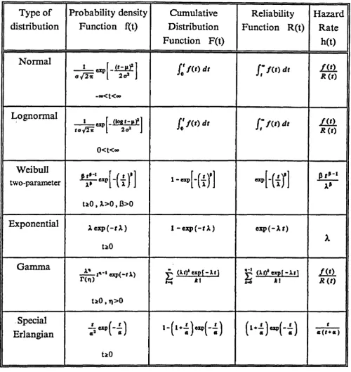
U S E F U L STA TISTICA L D ISTR IB U TIO N S

A number of statistical distributions have been used to model failure characteristics.

Table 2.1 summarises most of the more widely used distributions including those which

are applied more often in mechanical reliability assessment. The associated reliability

and failure functions, hazard rate, and the range of parameters variation are also listed.

(

2

)

(27)

Type of distribution

Probability density Function f(t)

Cumulative Distribution Function F(t)

Reliability Function R(t)

Hazard Rate

h(t)

Normal

— p = « P

oi]2n

-00<

[ - ( ' - F f l 2o*

t<°°

S it

W i t m .

* ( 0

Lognormal

1 cm (logl-p)2

SI

f W i t / V ( 0 dt / ( 0

t o j l i

0<

2 o*

t<oo

R ( 0

Weibull

two-parameter

UO , X>0, B>0

k*

Exponential _Aexp(-fX)

UO

1 -e x p (-f X) exp(-Xr)

X

Gamma

r ( n ) ,>

tiO , T)>0

£ (XD*expf-Xtl **n X1

g (X tfex p f-X il

W) ^ 1

m

j t ( o

Special Eriangian

UO

’-HM'i)

HM ’i)

«(»♦«)

t

Table 2.1 : Some Statistical Distributions Useful in Reliability Engineering.

(28)

A2

_A3

An

System

F igure 2.1 : R epresentation o f a Series System

A 1

A 1 A 1

(29)

Bn

An N n

A 1

N 2 B2

A 3 B 3 N 3

A 2

Figure 2.3 : Series System with Standby Redundancies

A1

A2

An

(30)

CHAPTER 3 LITERATURE SURVEY

The basic objective of the FMS concept is to achieve the efficiency and

utilization of mass production, while retaining the flexibility of a job shop - (ideally).

To achieve this goal, the production has to be well planned for an optimal run.

Machine loading and tool allocation is considered as the lowest level of production

planning problem. Both mathematical programming models and simulations are

employed to solve loading problems in FMS. A detailed study of the literature on

flexible manufacturing system as a whole was done before concentrating on the

problem. This literature review can be divided into five groups, namely tool life, tool

management, loading models, analogous systems, and reliability evaluations.

3.1 T ool Life :

To model a loading problem, it is important to assess the life of a cutting tool

during which the quality of the workpiece is acceptable. The ability to effectively assess

(31)

the ‘useful life’ of a tool would result in diminished inventory costs, optimal replenishing

policies, fewer machine stoppages for tool changes, and reduced workpiece rejects. A

tool is considered ‘failed’ when it either will not cut, or cuts in a manner grossly different

from a sharp tool. The failure may be caused due to a ‘single-injury’ or due to a

‘gradual wear*. In the manufacturing shops a tool has to be removed from service when

it produces unsatisfactory jobs, or routinely removed prior to this point, if its ‘economic

tool life’ is reached.

Gradual tool wear can be of various types, like flank wear, notch wear, crater

wear, edge rounding, etc. There has been no universally acceptable physical explanation

for tool failures. An empirical study assumes that even though various wear

mechanisms come into play, gradual wear is produced by temperature-dependent

mechanisms, and temperatures are greatly affected by cutting speeds. Taylor (1907),

developed the relationship between average tool life and cutting velocity, through an

empirical study of tool wear. His tool life equation is :

VTn = k o r

Where:

T actual tool life of the cutting time between resharpening (minutes);

16

(32)

V cutting speed (feet/minute);

n ,k empirical constant;

Heat generation increases with the increase in undeformed chip thickness and the

chip width. Cook (1973) provided an extension to the above relationship relating the

feed, speed, and depth of cut for a given tool life value, given a s :

K

= —

(4)

d * f >

Where

Vt equivalent cutting speed (feet/minute) for a given tool life;

f feed per revolution (inches);

d depth of cut (inches);

x, y, k empirical constants;

These equations provide the expected values for a gradual wear. Tool life

however, depends also on the arrival of ‘single-injury* events. The underlying physics

o f tool wear being so complicated, for general purposes, a failure rate function is best

(33)

Tool life being highly case sensitive, there have been extensive studies, under

varied conditions addressing the problem. For a rational design of a flexible

manufacturing system, the statistical variability o f tool life would provide a better

understanding of the system. The literature indicates that standard distributions such

as Normal, Log-normal, Weibull, Exponential, and Gamma distributions as well as

their combinations, can be justified and fitted to describe the life of a tool under varied

machining conditions.

Wagner and Barash (1971) reported that for high-speed steel turning tools the

tool life values are subjected to a statistical distribution which can be approximated by

a normal distribution. Based on experimental investigation, Hitomi et al. (1979) have

suggested that the log-normal distribution conform for the tool-wear distribution.

Friedman and Zlatin (1974) studied the tool life variation for several metal and cutting

tool-workpiece combinations. Jeng and Yang (1992) derived a tool replacement model

that took a general modelling approach to accommodate wider applicability. The

expected part dimension was assumed to be a nonlinear function which had its effect

from the cutting tool wear. The uncertain effects were aggregated together and treated

as a random error. The wear process was divided into three periods, the initial wear

period, the steady or normal wear period, and the accelerated wear period. Optimal

(34)

A noteworthy contribution to the study of tool life was provided by Ramalingam

and Watson in their three part publication. Ramalingam and Watson (1977), presented

the results obtained in cases where the useful life of a tool is terminated by a single

catastrophic injury. It was shown that for a time-independent degradation, the tool life

distribution can be given as an exponential distribution, or in other words a Weibull

distribution with shape parameter, p= l. In the case of time-dependent degradation, the

distribution obtained was a general Weibull distribution. So in general, the tool life

distribution for both time-dependent and time-independent failure hazards is given by

a Weibull distribution, and p is an indication of the time-dependence of the degradation

process. Ramalingam (1977) addressed the case where the tool is considered to

deteriorate by a gradual wear and cumulative wear process. The tool reaches the end

o f its life when a specified volume of material is removed from a relevant surface (flank

surface or rake face) of the tool. It was shown that in the linear wear regime, the

approximation o f the life distribution by a normal distribution is not, in most cases,

unrealistic. In the non-linear case the distribution was more log-normal. Whereas the

first and the second parts o f the publication used an arbitrarily introduced hazard

function to account for the distributed tool life, Ramalingam et al. (1978) showed that

the hazard function has a physical basis and is determined by the interaction between

the properties of the tool material and the characteristics o f the loading environment in

(35)

new hazard function obtained now, the tool-life distribution for single injury tool failure

was shown to be a Weibull distribution, thus showing the previous modelling to be

physically meaningful and realistic.

3.2 T ool Management :

It has been seen that the productivity of a FMS can be severely limited, without

an efficient and well maintained tool-management system. FMS being capable of

performing a wider variety of operations, poses the problem of being supplied by a

varied types of tools, at different times during the production run. Typically, the

flexibility o f an FMS is constrained by pallets availability and tool magazine capacity.

An effective tool management policy should thus,

✓ provide sufficient redundant tools at the machine, to take care of tool breakages

and/or tool wear.

✓ use preset tools to avoid larger and excessive tool inventory.

✓ maximize the variety of jobs that can be produced by the machine, under the

given resource constrains

✓ minimize the movement of tools between machines, during a production run,

(36)

Hankins and Rovito (1984) compared two tool allocation and distribution

strategies through a case study. It was seen that for the case in study, the tooling

strategy affected the number of machines required, the level o f manpower required, and

the level o f tooling inventory. The strategies compared were bulk exchange and tool

migration at the completion o f workpiece. As for the tool distribution, the bulk

exchange strategy was matched with manual loading and unloading of the machine

matrix, while the migration strategy was matched with automated loading and

unloading. The comparison study was done, using a Simulation. The data used as the

input was the data gathered from metal working industries using this kind o f systems.

Kiran and Karson (1988) noted that even after flexible manufacturing systems

became operational, tool management studies were not given sufficient attention. After

some financial disasters, both the FMS users and the machine tool builders recognized

that tooling can have a major effect on the performance of FMS. Usually an FMS is

used in a medium variety / medium volume manufacturing environment. Tool

management would be even more important and complicated, as the systems find their

application in a low volume/high variety environments. The objective o f an effective

tool management system is to provide the required tools to every operations on the

scheduled machine at the right time, so that the desired quantities o f workpieces are

(37)

Hedlund et al. (1990) used simulation to model the complex manufacturing

operations and controlling algorithms of a flexible manufacturing cell. The study was

done to compare the tool delivery system for an actual FMC being installed. Since parts

to be machined included hardened steel, some tool lives were foreseen to be as small as

5 minutes, which in turn demands a very effective tool management. The system

investigated consisted of seven CNC machines with a tool magazine of 50 or 68 tools.

In addition, there were two carousels, each having a capacity of 140 tools. An overhead

monorail robot was used for the tool transfers between the machines and/or carousal.

In advance of parts being brought to a machine for processing, the first five tools were

allocated, and the tool magazine was checked for those tools. Three delivery options

were debated. To help in analyzing the behaviour of the system, multiple output

statistic screens were developed to monitor the system during the simulation process.

The simulation identified the bottlenecks in the system.

Kolahan (1993) emphasised the need for the reliability analysis of the tooling

system in FMS. Reliability based models were developed to evaluate the tooling system

by its performance under different tooling strategies. The models determined an

optimal set of spares of required tools, so that the system attributes were optimized,

with the objectives o f minimizing the tooling cost and the occupancy of the tool

(38)

and permitted, thus quantifying the difference between the strategies, in terms of tooling

costs. The non-linear reliability constraints were linearized to form a linearized 0/1

integer model. A machine in the system could perform all the operations assigned to the

workpiece, as long as the required tools were available at the required time. A tool was

considered to be within its useful life, as long as the cumulative hazard function o f the

tool was less than the threshold. The value of the required reliability o f the system, and

hence the threshold value of the cumulative hazard was considered as a management

policy. Since the life time of the tools were less than the required operation time during

a production period, sufficient redundancies would have to be carried. More so,

because a workpiece could have only one process plan for its operations, or the best

process plan would have to be selected outside the model. A part entering the system

was loaded on a machine, where different tool types performed their operations, one

after the other. Therefore the problem could be treated as a series system, with standby

redundancies. A magazine was allowed to have a maximum of only five redundancies

o f a tool type, and the examples cited were suited to the assumption. However, the

individual tools were allowed to have any of the three failure distributions. The

research also included a model for reliability optimization. A search algorithm was

developed, which minimizes the tooling cost by a criterion of getting maximum

reliability improvement per unit cost. The procedure was repeated until the desired

(39)

3.3 L oading :

Stecke (1984) partitioned the FMS problems as Design, Planning, Scheduling,

and Control problems. Planning problems appear after the FMS is implemented, and

is in production. As a part of the planning problem, the part types have to be grouped

together, and have to be assigned to the available machines, along with the required

tools to process it, while ensuring that the resource constraints are not violated and that

the returns are maximized. This subset of activities is termed as loading. Loading is an

important component o f the overall FMS operational problem. Therefore, loading has

been the focal point of numerous research studies. Some of the salient literature has

been cited below. The literature has been divided into three groups, based on the

approach to the solution of the problem undertaken, i.e., analytical approach, heuristic

approach, and simulation approach.

3.3.1 A nalytical Approach :

Stecke (1983) defined five production planning problems that have to be solved

for efficient use o f an FMS. The problems being part type selection, machine grouping,

production ratio, resource allocation, and loading. The paper addressed the problems

(40)

formulated, and linearization methods were presented. For common problem sizes, the

problems were solved optimally, within a reasonable time.

Kusiak (1985) formulated a model that took into account the limitation o f the

tool magazine and the tool life o f individual tools. A 0/1 mixed integer linear program

was proposed. The model however did not consider the tool sharing between machines

or machine and tool cribs during the batch production. The life o f the individual tools

was assumed to be constant, independent o f the batches being processed.

Sarin et al. (1987) formulated a model addressing machine loading and tool

allocation problem. Given a fixed number o f parts, which are to be processed by a

group of machines, which have tool magazines loaded with tools o f limited life, the

objective was to minimize the total machining cost. The costs included both the cost o f

tool wear, and the cost o f machine usage. The model assigned the required tools to

machines, which stayed there for the entire planning period. Tool sharing between the

machines was not considered. The parts were to have a unique process plan, or the best

process plan was selected outside the model. A tool was used by the system for the

duration o f its useful life. Useful life o f a tool was a duration, determined by previous

statistics. An assumption that many tools and machines are not compatible drastically

(41)

Liang (1991) pointed out that when part selection and machine loading problems

are dealt with separately, and linked thereafter, they could contradict each other, and

lead to less meaningful, and sometimes even infeasible solutions. His study was directed

towards the concurrent part selection and machine loading decision problem. A model

was developed for a situation where the demand could vary widely, and tool sharing

was not possible between the machines or the tool crib. Individual tool life was assumed

to be shorter than the batch production time, necessitating the need for standby

redundancies within the machine’s magazine.

3.3.2 Heuristic Approach :

Berrada and Stecke (1986) considered a loading problem of simultaneously

assigning machine tools, operation, and cutting tools to the part types. An operation

is assigned to only one machine. Since balancing the workload corresponded to

m axim ising the production rate, the objective of the model was to balance the workload,

constrained by the tool magazine, machine tool, and system capacities. A non-linear

integer program was formulated, which was solved by a branch and bound algorithm.

O’Grady and Menon (1987) examined a master scheduling problem for an

existing FMS in Scotland. A multiple criteria approach was used to choose a subset of

(42)

orders for processing, subject to resource constraints and potentially conflicting

objectives. SCICONIC/VM mathematical programming system, running on a VAX

was used to solve the problem. The solution adopted a compromise philosophy. It was

argued that this solution procedure avoided the computational limitations associated

with the pursuit of a global optimality using a 0/1 integer model.

Ventura et al. (1988) developed two mathematical models to load tools to

machines in a FMS environment. Two sets of heuristic algorithms for solving the

models were presented. The objective functions were to minimize the time-span

required to process all the parts in a batch, and to minimize the number of part

movements required to process the overall batch of parts. Tool processing times were

considered to be machine dependent in one case, and machine independent in the other.

It was found that the effectiveness of these algorithms is very much dependent on the

magazine tightness values.

Part and tool movement policies are among the basic approaches used in loading

problems in flexible manufacturing systems. Han et al. (1989) addressed a problem of

loading a set o f tools to different machining centres, where each part visits only one

machine for its entire processing. Every machine could process all the operations on all

the part types, as long as the corresponding cutting tools are available. A tool required,

(43)

but not available in the machine’s tool magazine could be borrowed from other

machines. When the required tools to process a part are not mounted in the tool

magazine, either the part may be sent to another machining centre where those required

tools are available or the required tools may be transported from another machining

centre. Tool movement policy was seen advantageous. Since parts do not move, there

is no need to reposition the workpiece or recalibrate the position of the tool head which

results in higher cutting precision. Also, a part is processed by only one machining

centre. So a part is delivered into the shop only when a machining centre becomes

available, thereby resulting in less work-in-process. However, tool movement policy

results in tool-move delay time, which will be higher when the tool to be borrowed is in

use at the other machining centre. They proposed a non linear programming model for

the loading of a set of tools to the different machining centres, where each part visits

only one of the machining centres for its entire processing. The quadratic objective

function is to minimize the amount of tool traffic among the machining centres and

between a machining centre and tool crib. A heuristic solution method was suggested.

Analytical and simulated solutions were compared to the solution from the algorithm.

3.3.3 Simulation Approach :

One of the earliest study on loading FMS was done by Kathryn Stecke and

(44)

James Solberg. Stecke and Solberg (1981) performed their study in a practical

environment of ‘Caterpillar Tractor Company*. The system consisted o f eleven

production machines and an inspection machine. The operating strategies considered

involved policies for loading (i.e. allocating operations and tooling to machines) and

real time flow control. A detailed simulation was employed to test alternatives. The

results were different from those of classical job shop scheduling studies, showing the

dependence of system performance on the loading and control strategies chosen to

operate the flexible manufacturing system. A 0/1 non linear mixed integer model was

developed, which was solved by linearizing thereafter. This model did not consider the

finite life of the tools.

Carrie and Perera (1986) studied the effect of tool variety, product variety and

product similarity on the frequency of tool changes due to product variety, and due to

tool wear. They based their study on a particular FMS. It was found that the number

o f tool changes due to product variety is small compared to those due to tool wear. For

the analytical study they used the model given by Menon and O'Gradey (1984), with

some variations. They made a post-processor which reads a file of work flow d a ta , and

by referring to the part routing and tool requirement file, maintains a list of tools which

would be present in the tool magazine. Thus, the occurrence of tool changes due to

(45)

Gyampah et al. (1992) compared four scheduling strategies in the presence of

three part selection rules, through a simulation of a five-machine FMS tool handling

system. The strategies compared were bulk exchange, tool migration, resident tooling,

and tool sharing. Significantly different outcomes were seen between the different

strategies. Resident tooling was favoured over other strategies. It was pointed out that

the study used long cycle times of parts, and the results could be different when parts

with relatively shorter cycles were to be processed.

3.4 Analogous Literature :

Damodaran et al. (1992) developed models for production planning and cell

design in cellular manufacturing systems. Parts were allowed to have more than one

process plan, and the operation on the part could be performed on more than one

machine. Cells had an upper limit to the number of machines it could accommodate.

A model was developed to simultaneously form machine groups and to assign part-

operations to the selected groups. Penalty costs were imposed on inter-cell movements.

The non-linear constrain was linearized using the method suggested by Glover and

Woolsey (1973). The models developed were mixed integer linear models.

(46)

resource utilization, when part families and machine groups are formed simultaneously.

A part could have more than more than one process plan and each operation could be

performed on alternative machines. Integer programming models were developed,

considering budget, floor space and capacity of machines to study the effect of

alternative process plans and simultaneous formation o f part families and machine

groups on resource utilization. The non-linear constrain was linearized using the

method suggested by Glover and Woolsey (1973). In another case a model was

developed, that rearranged an existing manufacturing facility to Cellular

manufacturing.

Atmani et al. (1995) introduced a 0/1 integer programming model for

simultaneous solution of cell formation and operation allocation problem in cellular

manufacturing. A part is assumed to have more than one process plan, and each

operation could be performed on more than one machine. The objective of the model

was to simultaneously form machine groups and allocate operations of the part types,

so as to m inim ize the sum of operation, refixturing and transportation costs.

Precedence relations among the machines and machine duplications were not

considered. The model was used to solve large numerical examples . The model

(47)

3.5 Reliability Studies

It is possible to improve the reliability o f a system by improving the quality of

its components. However, beyond a certain point, the improvement of reliability per

unit cost may not be economical any more. Multiple copies may be beneficial or even

necessary if these components are used very often. Reliability could then be improved

by providing parallel paths, or standby redundancies. Predicting the number of spares

o f each component needed for a required operation time is of vital importance in

designing a new system. Optimizing the reliability of a system, by providing

redundancies has been the topic of many researches. Complex systems may contain

some components which fail more often. Determining the location and the number of

redundancies in the system is one of the issues discussed in this research.

Bellman and Dreyfus (1958) were among the first who applied dynamic

programming to the solution of the optimal redundancy problem. Their formulation

considered only two types o f constraints: cost and weight. Messinger and Shooman

(1970) conducted a tutorial review that evaluated and compared several techniques to

allocate the number of spares of each part type, to maximize the system reliability. For

an N-stage series system, Tillman et al. (1980) treated the problem of allocating

(48)

extension of this problem can be stated as finding the optimum number of redundancies

which maximizes the system reliability subject to cost constraints (Rao, 1992). Tillman

(1969) applied integer programming techniques to maximize the reliability or minimisra

the cost, subject to several constraints and the components may have different modes

o f failures. This required a bulky formulation that restricts the size of the system.

Hwang et al. (1971) applied a zero-one integer programming to minimize the weight of

sub-systems o f a life support system, subject to several nonlinear constraints while

maintaining an acceptable level of system reliability. Ghare and Taylor (1969)

determined the optimum number of redundant components in order to maximize the

reliability of series system subject to multiple resource restrictions. Solving the

associated zero-one programming model by a branch-and-bound procedure, they

showed that the optimal solution to the associated problem is equivalent to the optimal

solution for the optimal redundancy problem.

Pan et al. (1986) derived a mathematical model to predict the system reliability

of an automatic tool changing system, with the various cutting tools subject to Weibull

failures. The system was regarded as a series system with stand-by redundancies. A

recursive algorithm was presented to calculate the system reliability. The algorithm

permitted the use o f any failure distribution. However, no specific model to select the

(49)

combinations. They also took a numerical approach to integrate the reliability function

for each tool with different number of spares. Ghosh and Wells (1990) presented a

heuristic algorithm to solve the spares allocation problem to remote machines, in which

machines were subsystems of a series system that would be used only for a specified

period of time. They assumed that all spares must be assigned at the beginning of the

system’s mission. The algorithm determines number of spares for each subsystem

(machines) that maximizes the minimum probability of each machine consuming its

spares before the useful life of system is completed. To increase mean time between

failures and to improve system reliability, Sears (1990) proposed a top-down technique

to calculate required number of standby redundancies.

Kolahan (1993) in his thesis, emphasized the need for reliability studies on the

performance of an FMS. Tool sharing between the machines was taken into

consideration while modelling the problem. Also, a heuristic was developed to find the

optimum reliability for a given system. For reliability evaluations, the machining

centres were visualized as a series system, where the reliability of the system is the

product of all the sub-components (cutting tools) in the system.

There has been no literature that deals with a full loading problem, with

(50)

the production be carried out without interruptions, and without rejects of the work in

progress. This research aims at solving the loading problem, with reliability

considerations, thereby giving the production planner a comparison between the

(51)

CHAPTER 4 MODELS

This chapter presents a few models with various objectives, that would optimize

a typical loading problem in a FMS environment. The nomenclature and assumptions

used are defined. The layout of an FMS in consideration is shown. The analytical

model was run on packages LINGO® and LINDO®. The results obtained were verified

by comparing against the simulations done on GPSS/H® and WITNESS®. The

mathematical models were run on IBM® compatible PCs and SUN® workstation. The

simulations were run on IBM mainframe.

4.1 System Configuration :

The layout of the system configured is shown in Figure 4.1. The system although

hypothetical, is based on an existing system at Rock Island Arsenal, and presented by

Hedlund et al. (1990). The system consists of a number of machining centres (4 in the

(52)

the capacity to accommodate the batch to be processed. Parts enter and leave the

system by the common gangway. It is assumed that, in general, all the operations

required to be performed on a part can be done by a single CNC machines in the flexible

manufacturing system, as long as the required tools are available. The models, however,

can accommodate the need of restricting a particular tool or operation to specific

machines. Each machine has a tool magazine of a limited tool capacity. While the tools

are interchangeable between the machines, the tool magazines are fixed to the machine.

The tools are assembled in the collet and tool holders, in a tool room, and enter the

system through the tool transporter, or by a bulk exchange of the tool carousal. Since

the ‘useful life’ of a tool is less than the production period, tool magazines would have

to carry sufficient redundancies to process the entire demand without interruptions.

The tool transporter shown in Figure 4.1 is applicable to the models where tool sharing

is permitted. Tool transporter moves along a fixed path, as shown. Tool magazines of

all the machines are accessible to this transporter, during the production run. There can

also be a tool carousel within the system, which carries a larger number of tools, and is

accessible to the tool transporter, during the production run. This would permit the

system to hold more standbys of faster wearing tools, thereby allowing longer

production runs. Without any modifications to itself, the loading models developed

with tool change permitted, can accommodate the tool carousel. The total tool

(53)

to transport the tool to the recipient machine, the time to insert the tool into the

recipient machine’s tool magazine, and the time to carry the worn out tool away. Worn

out tools will be removed from the machine’s tool magazine during the production run,

and placed on the designated section of the tool carousal, as long as there is available

space in the carousal. In other words, the number of tools in the tool magazine of the

individual machine will be maximum at the beginning of the production run, and

(54)

4.2 Nom enclature :

Indices :

i : part type index, 1,2.... , /

j : machine index, (to) j 1,2,.... /

k : machine index, (from) k — 1,2,

1 : tool type index, 1 - 1,2 ,....,£

m : spares index, m - 0,l,....,Aff

P : process plan index p 1,2

For the models where tool sharing is permitted, index k denotes the machine

from which the tool is being borrowed, and index j denotes the machine to which the

tool is transported. For the models where tool sharing is restricted, index iris not used,

and the index j refers to the machine in context.

D ecision Variables :

Fraction of demand of part 7 \ processed on machine ‘j \ using

process plan *p \

1 if part 7* is processed on machine *j* using process plan *p \

(55)

1 if machine *j* has to be loaded with tool 7 ’.

Z j 1 0 otherwise.

1 if machine *j* has to be loaded by *m * spares of tool 7 \

\ 0 otherwise.

Nju Number of tools of type 7 ’ transported to machine *j* from 7 r \

N j Number of tools of type 7* mounted originally on machine *j*.

H j Number of tools of type 7* transferred from other machines to machine

Parameters :

1 if part 7* can be processed on machine *j* using process plan *p \

a ;._VP 1 0 otherwise.

1 if part 7 ’ can be processed using tool 7 ’ and process *p ’.

Pop ' 0 otherwise.

k Hazard rate of the tool with an exponential failure distribution.

Cj Unit cost of tool 7*.

Ej Tool magazine capacity available at machine *j\

M j Maximum number of tools of type 7 ’ that can be put on machine * j\

Demand for part 7 ’.

t^p Machining time for part 7 ’ using tool 7 ’, and process *p \

Ts Useful tool life available from each spare of tool 7* on machine *j*.

(56)

Time to insert a tool from machine ‘k for use on machine * j\

Q, Tool transporter time available during the production period.

Bj Machine time available, on machine * j\ during the production period.

Rm Reliability of tool type ‘7’ on machine *j* with *m ’ redundancies.

11^ Obtained reliability for part 7 \ on machine *j* using plan *p ’.

R j Reliability of tool type ‘7*.

Uj, Cumulative hazard factor of tool type *7\ on machine *j*.

(57)

tool In/out

tool changer tool carousel

o

tool m agazine'

•

machine machine

^ | I I f • •--- •-•v /* • • • • * .

ftool magazine 4 f tool magazine j pool magazine

4 . 7 T ‘ l N 1 • • +-T*

Local Queues

machine machine

parts

In-parts out«-=:

(58)

4.3 Assumptions :

While developing these models, the following assumptions were made to simplify

the modelling.

■a* The demand for each of the part type is known in advance, and will not change

during the production period.

» All the spares of a particular tool type are assembled to be identical.

«*■ Tool failures are independent of each other. So, the failure of one tool does

not affect the failure of another tool in the system.

« A machining centre can perform all the required operations of the assigned parts,

as long as the required tools are available in the tool magazine.

■a* Machining parameters such as feed, spindle speed, depth of cut, etc are determined

before the production run, and does not change during the production run.

The life of the tool transporter is much larger than the production period. So the

tool transporter has a constant reliability during this period.

«■ The tool life distribution of all cutting tools is exponential. But the mean would

depend on the tool type.

h* Stochastic, single catastrophic injuries to the tool are ignored.

» The detection of a tool failure is perfect.

(59)

4.4 Mathematical Modelling :

The purpose of the mathematical modelling is to optimize the loading problem

in a typical FMS. Layout of the system considered has been presented above. Tool

sharing, although economically advantageous for a large system, requires a more

complicated and meticulous tool setting and tool management systems, and additional

equipments. For a less flexible or a smaller system, the investment may not be worth

the returns. Thus an FMS may or may not have tool sharing. Two sets of

mathematical models have been developed. Each model considers two cases, one where

tool sharing is permitted, and the other where tool sharing is restricted.

4.4.1 Model I :

The objective of this loading problem is to minimize the tooling cost of the

system. Each tool type is given a fixed value of ‘useful life’. This value may have been

found from the statistical analysis of tool wear, in the past. The useful tool life is a

fraction of the absolute tool life, for a given tool type. Each machine has a tool

magazine, with a limited number of tool slots. Also, there is a limit on the machine

availability time during the production period. A demand can be split into batches, and

(60)

process plans. The optimal size of a batch is determined by the mathematical models.

4.4.1a Case 1, Tool Sharing N ot Allowed :

When tool sharing is not allowed, each machine will have to carry all the tool

types, and sufficient redundancies of each type to process all the batches scheduled for

the production period. The total number of tools in the magazine of a machine remains

constant throughout the production period. A tool type can be assigned to more than

one machine. The number of tool slots and the available time could be different from

machine to machine. A linear integer programming model developed, is presented

below.

J L Mjl

Minimize

£ J J m C,

Zjlm

(4 .1 )

j- 1 1*1 m* 0

Subject to

J P _{(4 .2 )}

V I

j*l p*i

L M

E E

m Z jlm * Ej (4.3)

(61)

£ £ PII P x lJ P ta P * h j £ V I J ( « )

i=l p=1 m*0

I P L

£ £ £ p a p X i j p ' u , * B J V J ( 4 5 )

i*l /?«! /-I

£ V = 1 V J . l (4.6)

m*0

Uj,

£ * V ■ ty,

m*=0

Integer Zjlm ^ j>l,m

GIN Xijp V i j \ p

(4 .7 )

is a 0/1 variable that indicates that a machine j has m spares of the tool type

7. Thus mZjto gives the number of spares of tool type 7, on machine j. Cj is the cost of

a tool o f type 7. The objective function therefore minimizes the total cost o f the cutting

tools. Constraint set 3.2 confirms that the sum o f the fractions of demand, named

batches, adds up to the total demand of each part type. Constraint set 3.3 ensures that

the total number o f spares, for all tool types assigned to a machine, is less than the

(62)

fraction is the batch size of part 1, designated to machine j to be processed by

process plan p. p is one, for all ilp combinations possible, and zero otherwise. Thus

constraint set 3.4 ensures that the usage of a tool of lj combination is less than the

available capacity. Constraint set 3.5 ensures that the available capacity of the

machining centres is not exceeded. For a machine j and tool type /, as m varies from 0

to MJy there can be only one , that can be 1. So, constraint set 3.6 sets a unique

number of spares for each tool type for all machines. Finally, J ^ h a s been defined as

a 0/1 integer variable.

4.4.1b Case 2, Tool Sharing is Permitted :

When tool sharing is permitted, all the tools within the system is available to

every machine in the system. However, the transport of tools from other machines

involves lost production time, for both the donor and the recipient machines. This

effect is quantified as a penalty cost of borrowing, and is included in the objective

function, which the program minimizes. This new configuration involves another

facility, the tool transporter. Along with the other capacity constraints mentioned in

the above model, this model also has to ensure that the available capacity, in terms of

time, of the tool transporter is not violated. Every time a required tool is brought in

FMS loading with reliability consideration.

Scholarship at UWindsor

Scholarship at UWindsor

FMS loading with reliability consideration.

FMS loading with reliability consideration.

FMS LOADING WITH RELIABILITY

CONSIDERATION

By

Abi M. Philipose

UNIVERSITY OF WINDSOR

To

God

ABSTRACT

TABLE OF CONTENTS

LIST OF TABLES

LIST OF FIG URES

CHAPTER 1

INTRODUCTION

CHAPTER 2

TERMS AND DEFINITIONS

(

)

S it

SI

m

’-HM'i)

HM ’i)

t

A2

A3

An

System

A 1

A1

A2

An

CHAPTER 3

LITERATURE SURVEY

K

= —

(4)

CHAPTER 4

MODELS

Minimize

£ J J m C,

Zjlm

E E

£ * V ■ ty,

_A3