Volume 8, No. 3, March – April 2017
International Journal of Advanced Research in Computer Science RESEARCH PAPER
Available Online at www.ijarcs.info
Happy sad demarcation from facial images using neural networks
Nivetha Yadhavan Department of Computer Science
Christ University Bengaluru, India
Nachamai M
Department of Computer Science Christ University
Bengaluru, India
Abstract: The aim of this paper is to discuss the development of an efficient neural network that demarcates primary emotions of humans such as happiness and sadness. The neural network implements a back-propagation algorithm that minimizes the error in the network, by traversing back in the network and rectifying the weights of the nodes in the layers of the neural network. The artificial neural network takes inputs in the form of co-ordinate pairs that constitute the facial fiducial points around the lips. The three pairs of points are the six input layer nodes. These nodes are connected to two nodes in the hidden layer which are connected to two output nodes. The output layer nodes are the results of the network and these nodes are binary. If the emotion is happy, the first node will be active having a value 1 while second node will be inactive having a value 0 and vice versa if the emotion is sad. Using the data generated by the algorithm the artificial neural network is trained. The paper also compares the effect of normalization in neural networks by comparing the confusion matrix for normalized input data and raw input data.
Keywords: Image analysis; Emotion Recognition; Neural Networks; Facial Images.
I. INTRODUCTION
Face recognition systems have contributed to various applications and are considered to be a major component of Human Computer Interaction (HCI). HCI is a major research field that encompasses cognitive sciences, human sciences, computational sciences and information technologies. It has emerged and evolved over three decades incorporating a variety of approaches from various disciplines. Facial expression detection, an extension of face recognition systems is one of the crucial requirements for making HCI more intelligent. The human face is vital when communicating both verbally and non-verbally as it is involved in all human communicative acts like facial expressions, speech and gesture. In contrast to the importance of faces, there has been relatively less work in the field of HCI involving faces and facial expressions, merely due to the technical difficulties and limitations involved. Facial expression recognition for a human is a very trivial activity but effective systems based on facial expression detection are very complex to design. A step prior to facial expression recognition is face recognition, which is an interesting application of pattern recognition. Entertainment, information security, and biometrics are some of the applications of face recognition [1]. Analogies that model the way humans approach recognition have given rise to neural networks, which have although developed from the biological roots [2]. Neural networks will make this easier by learning from the abundant data available in this field. Various approaches have been implemented in neural networks which include discrete cosine transformation (DCT), DCT is used to extract features from the high dimensional facial data [3]. A neural network is fed with available data and this data has pre generated output data set. These input/output sets are used for training and testing the neural network. The weights at the input-hidden layer connection and the hidden-output layer connection are adjusted to enhance the accuracy. The neural network learns from the training phase, this learning is applied to predicted results/outputs for the future inputs fed into the network. It is essential to enhance the network’s efficiency, this paper along with presenting a neural network using a mathematical model also targets in analysing the role of normalization in artificial neural networks.
II. LITERATURE SURVEY
algorithms/methods which involve mathematical calculations and statistical approaches. One method generates face candidates based on the spatial arrangement of skin patches by detecting skin regions over the entire image. The algorithm verifies each face candidate by constructing eye, mouth, and boundary maps [11]. This method is the detection of faces using color images. Another method is using Eigen faces [12]. Fiducial points are the characteristic feature points. When a face is considered there are a wide range of feature points around the eye, nose, and lips to name a few. For detecting happy and sad emotions the points around lip region is sufficient. An approach using geometric coordinates of the facial fiducial points, Euclidean distances and the differences in inter-feature distances fed into the neural network has shown 73% accuracy with the JAFFE database [13]. Neural networks are implemented using multilayer perceptron or convolution network [14]. Multilayer neural network with even a few hidden layers use arbitrary functions to approximate any measure from one-dimension space to another, this makes feed-forward neural networks a good universal approximator [15, 16]. Back propagation works faster than other approaches when classification is done using neural networks [17], and is proven to be more efficient [18], and these networks do not perform well when the input data ranges are large [19], the fiducial points of the face which can be given as input to the network are in coordinates and these will ideally be large values. Hence a normalizing procedure applied to this data might increase the efficiency of the neural network.
III. IMPLEMENTAION
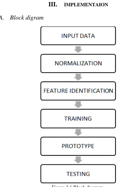
[image:2.595.38.228.373.675.2]A. Block digram
Figure 3.1 Block diagram
This paper discusses a neural network that is trained and tested to identify the emotion (happy/sad) of a person using facial fiducial points. The input to the network is three pairs of fiducial points around the lip region (ROI) and the output will be the emotion (happy/sad). The network has three layers, input, hidden and output. The input layer has six nodes (three pairs), the hidden layer has two nodes and the output layer has
two nodes. Back-propagation algorithm is used in the network to reduce the error in the network.
The neural network is fed with fiducial points (lip region) as its inputs. The proposed algorithm is applied to the inputs to generate outputs.
There are three phases in the network, they are, 1. Training phase
2. Testing phase 3. Prediction phase
I. Training phase
In this phase the network is fed with training dataset which has the inputs and the target outputs. The training phase is repeated for the given data for a number of specified times called the epoch.
An activation function is used to calculate the node values in the network. There are different types of activation functions; sigmoid, ReLU, LReLU are a few activation functions used in ANN systems. The activation function used in the proposed model is sigmoid.
Feed-forward recall
In layered network input vector z is mapped to output vector o. z is the input, o is the output and d is the desired output. In multilayer network there are internal mappings. Two layer networks,
o=T [WT [V2]], where T [V2] =y, internal mapping from input space z to internal output space y, where, W is the output layer matrix and V is the hidden layer matrix. The parameters for mapping z to ‘o’ are weights. The error is when o does not match d. This error is minimized by altering the weights.
Steps in Error back-propagation training
Step 1. Initialize weight vectors, w and v. Step 2. Starts with feed-forward recall phase. Step 3. Single pattern vector z is submitted as input. Step 4. Output vectors y and o are computed as, Step 5. y= [Vz]
Step 6. o= T[Wy]
Step 7. Error signal computation phase
Step 8. First the error is computed for the output layer, then the network nodes
Step 9. The weights are adjusted Step 10. First the W matrix (output layer) Step 11. Then the V matrix (hidden layer)
Step 12. The learning stops when the error is less than the upper bound, Emax
Step 13. If error is greater than Emax, run the cycle again, else stop.
II. Testing phase
B. Data Set
Figure 3.3 Snapshot of the data set
This research uses the Grammatical Facial Expressions Data Set [20] which is composed of data from eighteen videos. The data set has 1062 samples each having 99 features, which are 3 dimensional coordinate points. The x and y coordinates are given in pixels, and the z coordinate is given in millimetres. These pixels are the facial fiducial points on a human face; the areas of interest in this dataset are eyes, eyebrows, nose, nose tip, mouth, face contour and iris. From these 99 attributes the implementation presented in this paper considers six fiducial points from the mouth region which are used in the mathematical model to identify if the person is smiling or not. The points considered are around the lips; left corner, right corner and lower middle points. From the dataset, it can be found that the three that are needed for the model are 48, 54 and 62 in the dataset. These points are separated from the other points.
Points 48 and 62 are the endpoints of the lips, the average distance between these points and the minimum and maximum distances are calculated to find the threshold value for the algorithm.
C. Preprocessing
The input data is preprocessed by extracting only the coordinates that the network requires. The extracted data is normalized and to find the difference in the performance and accuracy of the network. Normalization techniques are implemented to increase the efficiency of the neural network. The normalization applied reduces the range of the input values as neural networks work better for smaller values. The data used is normalized in two steps:
• Standardizing • Scaling
Standardizing brings the data to the range 0 to 1 by using the formula:
x_std=(x-x_min)/(x_max-x_min) (i) where x is the input data,
x_std is the standardized value,
x_min is the Minimum value in x values, x_max is the Maximum value in x values,
Scaling scales the values in the given range, the range used here is -1 to 1(most efficient range for artificial neural networks; this range prevents saturation of weights, i.e., the values do not converge). Scaling uses the formula:
x_scaled=x_std*(∂_max-∂_min)+ ∂_min (ii) where, x_scaled is the scaled value,
x_std is the standardized value ∂_min is the Minimum range ∂_max is the Maximum range
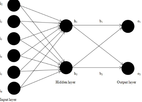
[image:3.595.319.553.128.295.2]D. Algorithms
Figure 3.2 shows the neural network that is implemented in this system which has six input nodes, two hidden nodes and two output nodes.
Figure 3.2 Architecture of the neural network for the proposed system
1. The back propagation algorithm:
Step 1: Initializing the variables Six inputs (i1, i2, i3, i4, i5, i6) Two outputs (o1, o2)
Two bias nodes (b1, b2)
Hidden layer neurons (h1_out, h2_out) - ∑ (w*i) (h1_net, h2_net).
The resultant values of activation function on h1_net and h2_net are h1_out and h2_out.
(o1_net, o2_net) are the summation of the hidden layer nodes.
(o1_out, o2_out) are the results of activation function on o1_net and o2_net.
(w1-w6) are the weights from input layer to hidden layer and (w7-w12) are the weights from hidden layer to output layer. These weights are initialized to uniformly distributed random values in the range 0 to 1.
eta is the learning rate.
Step 2: Forward pass
Find (h1, h2) net, (h1, h2) out, (o1, o2) net and (o1, o2) out.
Find errors for each output as (t-o). Find the total error for the network.
Step 3: Backward pass • Output layer
Find the change: - ∂Etotal/∂wi (iii) ∂Etotal/∂wi=∂Etotal/∂o1_out*∂o1_out/∂o1_net*∂o1_net/∂ wi
Using this Etotal value the new weight is found by calculating,
wi_new=wi-(eta*∂Etotal/∂wi) (iv) Similarly, the error for all the output layer nodes is found and used to correct the weights of the output layer.
Next, continue the backwards pass by calculating new values for the hidden layer weights.
Find the change: - ∂Etotal/∂wi (v) ∂Etotal/∂wi=∂Etotal/∂h1_out*∂h1_out/∂h1_net*∂h1_net/∂ wi
Using this Etotal value the new weight is found as, wi_new=wi-(eta*∂Etotal/∂wi) (vi) Here,
∂Etotal is the total error calculated,
∂wi is the weight of the ith
node.
A similar process is used for the hidden layer as well, but since the output of each hidden layer neuron contributes to the output (and therefore error) of multiple output neurons a slightly different process is done here. It is evident that h1_out affects both o1_out and o2_out since these results are carried forward in the network. The result of the hidden layer is used to find results in the output layer; therefore, the
∂Etotal/∂h1_out needs to take into consideration its effect on
both the output neurons:
∂Etotal/∂h1_out=∂Eo1/∂h1_out+∂Eo2/∂h1_out (vii)
Starting with ∂Eo1/∂h1_out:
∂Eo1/∂h1_out=∂Eo1/∂o1_net*∂o1_net/∂h1_out (viii)
This way the new weights for the hidden layer nodes are found.
Using these new weights feed forward the network again. In every iteration, the error decreases and the actual output moves closer to the target output.
2. Happy sad demarcation algorithm
This model uses three points around the lip region; left corner of the lips (A), right corner of the lips (B) and the middle point on the lower lip (C). These values are used to find the angle made by the lines AC and BC. This angle changes when the person smiles and hence is used to identify if the person is smiling or not.
Step 1: Input data (six feature points)
Step 2: Consider the line from the left corner to the lower middle point and the line from the right corner to the lower middle point.
Step 3: Find the angle between these two lines.
Step 4: If the angle is greater than 18.68 the person is happy, otherwise the person is sad.
18.68 is the threshold value which is obtained by processing 40 sample images of 10 subjects (2 images of each subject for each emotion).
E. Result
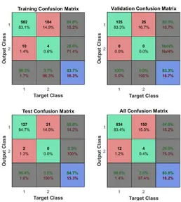
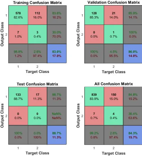
Confusion matrix gives a set of factors using which the performance and efficiency of the network can be discussed. True positive, true negatives, false positives and false negatives are the four main factors to be derived from a confusion matrix to analyze the network. For the network presented in this paper it is considered that happy is positive and sad is negative. Therefore, true positive is when target and actual outputs are happy, true negative is when target and actual outputs are sad, false positive is when target output is sad and actual output is happy and false negative is when the target output is happy and actual output is sad. Figure 3.4 shows the confusion matrix of the neural network for raw data (not normalized), and the Figure 3.5 shows the confusion matrix of the neural network for normalized data inputs. In the
matrices shown, the cells [1,1] and [2,2] show the number and percentage of correct classifications, the cells [1,2] and [2,1] show the number and percentage of incorrect classifications. The cells [1, 3] and [2, 3] give the percentage of correct classifications and incorrect classifications for the total records taken in the respective row. The cells [3, 1] and [3, 2] give the percentage of correct classifications and incorrect classifications for the total records taken in the respective column. The cell [3, 3] gives the percentage of correct classifications and incorrect classifications for all the records taken.
Table 3.1 Raw data Factors Training
Phase
Testing Phase
Overall Results True Positive 83.1% 84.7% 83.4%
True Negative 0.6% 0.0% 0.4%
False Positive 1.4% 1.3% 1.2%
False Negative 14.9% 14.0% 15.0%
Table 3.4 Normalized data Factors Training
Phase
Testing Phase
Overall Results True Positive 82.6% 88.7% 83.9%
True Negative 0.4% 0.0% 0.4%
False Positive 1.0% 0.0% 0.7%
[image:4.595.307.565.383.670.2]False Negative 16.0% 11.3% 15.0%
Figure 3.5 Confusion matrices for normalized input data
F. Conclusion
The importance of normalization is evident after analyzing the network for the proposed mathematical model by considering the confusion matrices generated. The overall accuracy of the network for raw (not normalized) input data is 83.8% and the same for normalized input data is 84.3%. There is a 1.5% increase in the efficiency of the network when the input is normalized. This shows that neural networks are trained better and give increased efficiency in terms of performance when the input data is normalized before feeding it to the network.
IV. REFERENCES
[1] Nandini, M., P. Bhargavi, and G. Raja Sekhar. "Face Recognition Using Neural Networks." International Journal of Scientific and Research Publications, Volume 3, Issue 3, (March 2013).
[2] Ripley, Brian D. Pattern recognition and neural networks. Cambridge university press, first paperback edition published 2007.
[3] Delipersad, S. C., and A. D. Broadhurst. "Face recognition using neural networks." Communications and Signal Processing, 1997. COMSIG'97., Proceedings of the 1997 South African Symposium on. IEEE, (1997).
[4] Dr. Nachamai M, Pranti Dutta “Demarcating Happy Affect Identification in Faces Using a Mathematical Model,” Demarcating Happy Affect Identification in Faces Using a Mathematical Model, Volume 2, Issue 5, (October 2014). [5] Kjeldskov, Jesper, and Connor Graham. "A review of mobile
HCI research methods." International Conference on Mobile Human-Computer Interaction. Springer Berlin Heidelberg, LNCS 2795, (pp. 317-335, 2003).
[6] F. Karray, J. A. Saleh and M. N. Arab “Human-computer interaction: overview on state of the art,” International Journal on Smart Sensi and Intelligent Systems, Volume. 1, Issue 1, (2008).
[7] Chibelushi, Claude C., and Fabrice Bourel. "Facial expression recognition: A brief tutorial overview." CVonline: On-Line Compendium of Computer Vision 9 (2003).
[8] X. Lu, “Image analysis for face recognition,” Publisher: Citeseer, (2003).
[9] H. Fatemia, H. Corporaal, T. Basten, P. Jonker and R. Kleihorst “Implementing face recognition using a parallel image processing environment based on algorithmic skeletons”, (2009). [10] B. K. Gunturk,A. U.Batur, Y. Altunbasak, M. H. Hayes and R. M. Merserereau “Eigenface-domain super-resolution for face recognition,” JIEEE Transactions on image processing, Volume. 12, Issue. 5, (2003).
[11] Hsu, Rein-Lien, Mohamed Abdel-Mottaleb, and Anil K. Jain. "Face detection in color images." IEEE transactions on pattern analysis and machine intelligence, Volume 24, Issue 5 (2002), pp 696-706.
[12] Jamil, Nazish, S. Lqbal, and Naveela Iqbal. "Face recognition using neural networks." Multi Topic Conference, 2001. IEEE INMIC 2001. Technology for the 21st Century. Proceedings. IEEE International. IEEE, (2001).
[13] Lawrence, Steve, et al. "Face recognition: A convolutional neural-network approach." IEEE transactions on neural networks, Volume 8, Issue 1 (1997), pp 98-113.
[14] M. Gargesha, P. Kuchi, and I. D. K. Torkkola. Facial expression recognition using artificial neural networks. In EEE 511: Artificial Neural Computation Systems, (2002).
[15] Hornik, Kurt, Maxwell Stinchcombe, and Halbert White. "Multilayer feedforward networks are universal approximators." Neural networks , Volume 2, Issue 5 (1989), pp 359-366.
[16] Hornik, Kurt. "Approximation capabilities of multilayer feedforward networks." Neural networks, Volume 4, Issue 2 (1991), pp 251-257.
[17] Back propagation <http://neuralnetworksanddeeplearning.com> [18] Shamsuddin, Siti Mariyam, Md Nasir Sulaiman, and Maslina
Darus. "An improved error signal for the backpropagation model for classification problems." International Journal of Computer Mathematics, Volume 76, Issue 3 (2001), pp 297-305.
[19] Krizhevsky, Alex, Ilya Sutskever, and Geoffrey E. Hinton. "Imagenet classification with deep convolutional neural networks." Advances in neural information processing systems. 2012.