U s i n g D e c i s i o n T r e e s t o C o n s t r u c t a P r a c t i c a l P a r s e r
M a s a h i k o H a r u n o * S a t o s h i S h i r a i t Y o s h i f u m i O o y a m a i m h aruno({i'ldl).at.r.co.jt) sld rai'(i'cs]al).k(~cl.n|,t.co.jl) o o y a l na.(.~}csla I).kccl.nl, t..co.j p* A'I'I{ l h t m a . n In r e t i n a . l i o n I ' r o c c s s i n g R e s e a r c h L a b o r a t o r i e s 9_9 l l i k a r i d a i , S '~d~a.-cho, S o r a k u - g u n , K y o l ; o 6 1 9 - 0 2 , J a p a n
* N T T C o m m u n i c a t i o n S c i e n c e l , a b o r a t o r i e s
2-4 l t i k a . r i d a i , S A k a - ( h o , S o r a k u - g u n , K y o t o 6 1 9 - 0 2 , 3 a p a n .
A b s t r a c t
This l)al)er describes novel and practical .lal)anesc parsers that uses decision trees, l"irst, we COl> struct a single, decision tree to estimate modifica-- lion probabilities; how one phrase tends t.o modify another. Next, we introduce a boosting algorithm in which several decision t.rees are COllst.ructed and then combined for probalfility estiinat.ion. 'lThe two constructed parsers are evalua.ted I)y using the El)t{ .Japanese annotated corpus. The single-tree method outperforlns the conventional Japanese stochastic reel.hods by 4%. Moreover, the boosting version is shown to h;we significant adwmtages; 1 ) better pars- ing accuracy than ils single-tree counl.erparl for any alnoullt o[" training data and 2) no over-titling 1o data. for va.rious iterations.
1 I n t r o d u c t i o n
Conventional parsers with practical levels of per f o r mance require a number of sophisticated rules that. haw" to be hand-crafted by human linguists. It is time-consuming and cumbersome to mainl.ahl tltese rules for two reasons.
* The rules are specific to the application domain.
* Specific rules handling collocat.ional expressions create side effects. Such rules often deteriorate the overall performance of the parser.
q'he stochastic approach, on the other hand, has the potential to overcome these difficulties. Because il induces stochastic rules to maximize ow~'ra.ll per- ['onnance against t.raining data, it. llOf Ollly adapts to any application domain but also may avoid ow>r- fitting to the data. In the late 80s and early 90s, lhe induction and parameter estimation of l)robabilis - tie context, free grammars (PCF(',s) from corpora were intensively studied, la;ecause these grammars comprise only nonterminal and part-of-speech tag symbols, their performances were not enough to be used in practical applications (Charniak,
1993).
Abroa.der range of information, in lmrticular lexical in- forinatiolq was tbund to be essential in disambiguat- ing the syntactic structures of real-world sentences. SI'ATTEt{ (Magerman, 1995) augmented the pure
I'(:I"G by introducing a. mnnl)er of lexical at.tributes. The parser controlled applications of each rule by us- ing the lexical constraints induced by decision tree algorithnl (Quinlan, 1993). rFhe SI)N]'TEt{ parser attained 87% accuracy and first made stochastic parsers a practical choice. The other type of high-
precision parser, which is based on dependency ana[- 5'sis was introduced by Collins (Collins, 1996). l)e-
pendency a.mdysis first, segments a sentence into syn- tactically meaningful sequences of words and then considers the modificatioll of each segment. Collins" parser computes the likelihood that each segment modifies the other (2 term relation) by using large corpora. These moditication probabilities are con- ditioned by head words of two S{"glnelltS, distance between the two segments and otlmr syntactic %a- tures. Although these two parsers have showll silni- lar performance, the keys of their success are slight ly diflk~renl.. SPA'[.'TER parser perforlnanee greatly de- pelldS on the feat.tire sehection ability of the decision tree algorithm rather than its linguistic representa- tion. On t, he other hand, dependency analysis plays an essential role in Collins' parser for elficienlly ex- tracting inK)rmation from corpora.
In lifts i)al)er, we (lescribe practical .]apanes(" de- pendency parsers that uses decisio11, trees, in the .lal)anese language, dependency analysis has I)ecn showll to ])e powerful because seglllellI (bullselsll) order in a sentence is relal:ively free compared to l!',uropean languages. Japanese dependency parsers generally proceed in three steps.
l. ,qeglnent a sentence into a sequence of t)unsetsu.
2. Prel)are a modification matrix, each value of which rel)resents how one ])/illSet.Sll is likely to modify another.
3. Find optimal modifications in a sentence by a dynanfic progranmfing technique.
Stochastic dependency parsers like Collins', on the other hand, define a set of attributes for condition- lug the modification probabilities. Tile parsers con- sider all of the a t t r i b u t e s regardless of bunsetsu type. These m e t h o d s can encompass only a small n u m b e r of features if the probabilities are to be precisely evaluated from finite n u m b e r of data. Our decision tree m e t h o d constructs a more sophisticated modi- fication matrix. It. automatically selects a sufficient number of significant attributes according to bun- setsu type. We can use arbitrary numbers of the attributes which potentially increase parsing accu- racy.
Natural languages are full of exceptional and collo- cational expressions. It is ditfieult for machine learn- ing algorithms, as well as h u m a n linguists, to judge whether a specific rule is relevant in terms of over- all performance. To tackle this problem, we test the mixture of sequentially generated decision trees. Specifically, we use the Ada-Boost algorithm (Ere- und and Schapire, 1996) which iterat.ively performs two procedures: 1. construct a decision tree based on the current d a t a distribution and 2. u p d a t i n g the distribution by focusing on d a t a t h a t are not well predicted by the constructed tree. T h e final modification probabilities are computed by mixing all the decision trees according to their performance. T h e sequential decision trees gradually change from broad coverage to specific exceptional trees t h a t can- not be captured by a single general tree. In other words, the m e t h o d incorporates not only general ex- pressions but also infi'equent specific ones.
T h e rest of the p a p e r is constructed as follows. Section 2 summarizes dependency analysis for the J a p a n e s e language. Section 3 explains our decision tree models t h a t c o m p u t e modification probabili- ties. Section 4 then presents experimental results obtained by using E D R J a p a n e s e annotated corpora. Finally, section 5 concludes the paper.
2
D e p e n d e n c y A n a l y s i s in
J a p a n e s e
L a n g u a g e
This section overviews dependency analysis ill the J a p a n e s e language. Tile parser generally performs the following three steps.
1. Segment a sentence into a sequence of bunsetsu.
2. P r e p a r e modification matrix each value of which represents how one bunsetsu is likely to modify the other.
3. Find optimal modifications in a sentence by a dynamic p r o g r a m m i n g technique.
Because there are no explicit delimiters between words in Japanese, input sentences are first, word segmented, part-of-speech tagged, and then chunked into a sequence of bunsetsus. Tile first step yields, for the following example, the sequence of bunsetsu
displayed below. The parenthesis in tile J a p a n e s e expressions represent the internal structures of the bunsetsu (word segmentations).
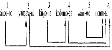
E x a m p l e : tl~g H (D/Y)i[Z~P)r'(D-J"~ ~ 4o 7~"7 4 > ~ ' ~ / v / ' ~
((~H)(e))) ((Y;k-)(l:))((~)(©))
kinou-no yuugata-ni ki~u'o-t~o yesterda~NO et,enit~y-NI neighbor-No((~k
S)(~),)) ((
v 4 >
)(~))
((~):/~)(tZ)
kodom(>ga wain-wo r~omu+ta childrcr~-GA w i n e - W O drit~k+PAST
T h e second step of parsing is t.o construct a modifi- cation matrix whose values represent the likelihood t h a t one bunsetsu modifies another in a sentence. In the J a p a n e s e language, we usually make two as- sumptions:
1. Every bunsetsu except, the last. one modifies only one posterior bunsetsu.
2. No modification crosses t.o other modifications in a sentence.
Table 1 illustrates a modification m a t r i x for the e x a m p l e sentence. In the matrix, co]unms and rows represent anterior and posterior bunsetsus, respec- tively. For example, the f r s t bunsetsu 'kinou- no" modifies the second 'yuugala-7~i'with score 0.70 and the third 'kil~jo-~o'with score 0.07. T h e aim of this p a p e r is to generate a modification m a t r i x by using decision trees.
k m o u - n o
yu~gala, nt 0 . 7 0 y u ~ g a ~ a - n ,
klnjo-no 0 . 0 7 0 . 1 0 L'lnjo-no
kodorno.ga 0 . 1 0 0 . 1 0 0 . 7 0 kodoHio*ga
~l, ain-wo 0 , 1 0 O . 1 0 0 . 2 0 0 . 0 . 5 ~'a~T~-u,o
71orllu-oa 0 0 3 0 . ' 7 0 O . I O 0 . 9 5 I O 0
'/Fable 1: Modification Matrix for Sample Sentence
T h e final step of parsing optimizes the entire de- pendency structure by using the values in the mod- ification matrix.
Before going into our model, we introduce the no- tations t h a t will be used in the model. Let. ,5' be the input sentence. S comprises a bunsetsu set. B of length m ({< b~,f~ > , . . . , < b , , , f , , > ) ) in which bi and J'i represent the ith bunsetsu and its features, respectively. We define D t.o be a modification set; D = { m o d ( l ) , - . . , m o d ( , n - l)} in which rood(i)indi- cates tim n u m b e r of busetsu modified by the ith bun- setsu. Because of the first assumption, the length of D is always m - 1. Using these notations, the result of the third step for the example call be given as D = {2, 6, 4, 6, 6} as displayed in Figure 1.
3
D e c i s i o n T r e e s for D e p e n d e n c y
A n a l y s i s
3.1 S t o c h a s t i c M o d e l a n d D e c i s i o n T r e e s
1
kin0u-n0 yuugat
3
4
ni kinj n0 k0d0m ga
_ll
5
ain-w0 n0mu.t
Figure 1: Modification Set for Sample Sentence
terms of the training da.ta distribution.
D b . , =
P(Z)IS) =
P(Z)IB)
By assuming the independence of modifica-
tions, P ( D I H ) can be t r a n s f o r m e d as follows. P ( y e s l b i , bj , f ~ , . . . , f ,, ) means the probability t h a t a pair of bunsetsu bi and bj haw" a modification rela- tion. Note t h a t each modification is constrained by all f e a t u r e s { f ~ , . . . , f m } in a sentence despite of the assumption of independence.tNe use decision trees to dynamically select a p p r o p r i a t e features for each combination of bunsetsus fi'om {f~ , . . . , f,,, }.
f'(1)[l,) =
1 - I l ' ( g , b s , f , , . . . , f ,, )l,et us first consider tit(.' single tree case. T h e lraining d a t a for the decision tree comprise any un- ordered combination of two bunsetsu in a sentence. Features used for learning are the linguistic informa- tion associated with the two bunsetsu. T h e next sec- tion will explain these features in detail. T h e class set for learning has binary values yes and no which delineate whether the data (the two bunstsu) has a moditication relation or not. In this setting, the decision tree algorithm automatically and consecu- tively selects the significant Datures for discriminat- ing m o d i f y / n o n - m o d i f y relations.
We slightly changed C4.5 (Quinlan,
1993)
pro-grants to be able to e x t r a c t class Dequen- d e s at every' node in the decision tree be- cause our task is regression rather than classi-
fication. 13y using the class distribution, we
conllmte the prol)ability l ' o T ( y e s l b i , bj, J'~ , . . . , f ,n) which is the Laplace estimate of empirical likeli- hood t h a t bi modifies bj in the constructed deci- sion tree D T . Note that it. is necessary to nor- malize P D W ( y e s l b i , b j , f , , . . . , f m ) to a p p r o x i m a t e P ( y e s [ b i , b j , f ~ , . . . , f m ). By considering all can- didates posterior to hi, P ( y e s l b i , bj, f ~ , . . . , f r o ) is c o m p u t e d using a heulistic rule (1). It is of course reasonable to normalize class frequencies instead of the probabilit.y P o T ( y e s l b i , bj, , f ~ , . . . , fro). Equa- tion (1) tends to emphasize long distance dependen- cies more than is true for frequency-I)ased normal- ization.
P ( y c s l b i ,bj, f ~ , . . . , f, ,, ) ~_
P D T ( y e s l b i , bj, f ~ , . . . , f ,, )
(1) k >i"' P DT(yeslbi, bj , f ~ , . . . , f m )
Let us extend the above to use a set of decision trees. As brietty mentioned in Section 1, a n u m b e r of infrequent and exceptional expressions a p p e a r in any natural language phenomena; they deteriorate the overall p e r f o r m a n c e of apl)lication systems. It is also difficult for a u t o m a t e d learning s y s t e m s to detect and handle these expressions because excep- tional expressions are placed in the same class as frequent ones. To tackle this ditficulty, we gener- ate a set of decision trees by a d a b o o s t (Freund and Schapire, 1996) algorithm illustrated in Tabh-. 2. T h e algorithm first sets the weights to 1 for all exam- pies (2 in Table 2) and repeats the following two procedures T times (3 in Table 2).
1. A decision tree is constructed by using the cur- rent weight vector ((a) in Table 2)
2. E x a m p l e d a t a are then I)arsed by using the tree and tim weights of correctly handled e x a m p l e s are reduced ( ( b ) , ( c ) i n Table 2)
1.
3.
I n l m t : sequence of N examples < c,, w, >, ..., < eN, WN > in which ei ~1.11(| Wz represent. ~11 exalKlple and its weigld, respectively.
I n i t i a l i z e the weight vector w, =1 for i = 1 . . . ~,r Do f o r t = I , ' 2 , . . . , T
(a) Call C.t.5 providing it wilh |he weight vcclor w,s attd C o n s t r u c t a modification l)robability
set, ht
(b) Let. E r r o r be a set of examples that are not ident.itied by ht
Compute the pseudo error rate of ht:
( t -~- E iCE,.,.o,.Wi/ E i=aN wi iI'{t > }, t h e n abort loop
l ~ e t
(c) For examples correctly predicted by h t, update the weights vector to be wi = II'i/~t
4. O u t p u t a fill~tl probability set.:
hf = E ,=, 7 ~ /Jr z ' ' ' ~ l t = . . l o Y ~ t )
,'(
Table 2: Combiniug 1)ecisiou Trees by Ada-boost Algorithm
Tile final l)rol)ability set h j is then comfmted
by mixing T trees according to their perfor-
mance (4 in Table 2). Using h r instead of
P o T ( y e s [ b e , bj, f , , . . . , f , , , ) , in equation (1) goner- ates a boosting version of the dependency parser.
3 . 2 L i n g u i s t i c F e a t u r e T y p e s U s e d f o r
L e a r n i n g
[image:3.612.88.271.53.135.2] [image:3.612.313.546.255.557.2]1 lexical information of head word
2 part-of-speech of head word
3 type of bunsetsu
4 p u n c t u a t i o n
5 parentlmses
Table 3: Linguistic Feature T y p e s Used for Learning
6 distance between two bunsetsu
7 particle 'wa' between two bunsetsu
8 p u n c t u a t i o n between two bunsetsu
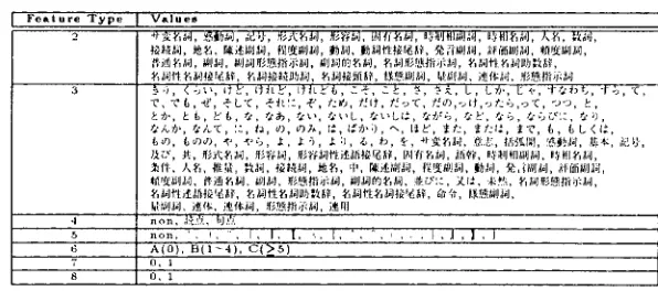
F e a t u r e T y p e V a l u e s
gJ~ga=], }~lJ].J. N0a,]lt.~f~m)l-;a,]. ~itja.jfl~-,t.]. ~',.l#]ft~,*al{mij~,~], g.~.]'I~gj,;}ll)fi.~:,~i'.
&~', & 6, ~P'l~, ta', f~'$~, t.¢~., ~ ' ~ ' L , fd~.~Ll~, ~]fiG, t,.~' fdG, ~'GC¢:2, ta'~l,
**']J)', fa'/~', ::, fa, a), tO.g, {~*, l.*~),;),--., lt~', ~t:, ~t:t*-, ~[-~, ~a, 6 L < { / , 6,,% 6¢1a), ~-., < ' b , . t . . 1 : 5 , .t:!, &, ab, ~ . ~t~£.l.}. 0:.&:, t,~,f~l, '~,M.]. l£V.. ,El). -~fl:. Ale,, IlU~I, Ira4, ¢g,~¢~,4, tRI'~, q,, ~jtd.{~l,tsj. l'~iI[,~Ja.I. ~/~,'0J, ~,{hllja4, ,i.l:fllfi/g]aaJ,
n o n , a:~."L, t,JfL
n o n , ' , q, , 1 , I , [ , ' , . l , ' , " , , , , , l , l , ] , I
7
8 0 , 1
" g r a p h dBt"
A(o), B ( l - 4 ) , c(>,5)
O , 1
Table 4: Values for Each Feature T y p e
84
8 . 3 5
83
82 5
82
Two Bunsetsu
~
Others
s o o o l o o 0 o l s o o o 2 0 0 0 0 2 5 o 0 o a o o o o a s o o o 4 o 0 o o 4 5 o 0 0 s o o o o N u m b e r o l Training D a t a
Figure 2: Learning Curve of Single-Tree Parser
the two bunsetsu constituting each data. Tile class set consists of binary values which delineate whether a sample (the two bunsetsu) have a modification re- lation or not.. We use 1"3 features for the task, 10 di- rectly fi'om the 2 bunsetsu under consideration and 3 for other bunsetu information as SUlnmarized in 'Fable 3.
Each bunsetsu (anterior and posterior) has the 5 features: No.1 to No.5 in Table 3. Features No.6 to No.8 are ]'elated to bunsetsu pairs. Both No.1 and No.2 concern the head word of the bunsetsu. No.1 takes values of frequent words or thesaurus cat- egories (NLRI, 1964). No.2, on tile other hand, takes values of part-of-speech tags. No.3 deals with bun- setsu types which consist of functional word chunks or the part-of-speech tags t h a t dominate the bun- setsu's syntactic characteristics. No.4 and No.5 are
binary features and correspond to p u n c t u a t i o n and parentheses, respectively. No.6 represents how m a n y bunsetsus exist, between the two bunsetsus. Possible values are A(0), B ( 0 - - 4 ) and C(>_5). No.7 deals with t.he post-positional particle ' w a ' which greatly inttu- ences the long distance dependency of s u b j e c t - v e r b modifications. Finally, No.8 addresses the punct.ua- t.ion between the two bunsetsu. T h e detailed values of each feature type are summarized in Table 4.
4
E x p e r i m e n t a l R e s u l t s
We evaluated the proposed parser using the E D R J a p a n e s e a n n o t a t e d corpus (EDR, 1995). T h e ex- p e r i m e n t consisted of two parts. One evaluated tim single-tree parser and the other the boosting coun- t.erpart. In the rest of this section, parsing accuracy refers only to precision; how m a n y of the s y s t e m ' s o u t p u t are correct in t.erms of the a n n o t a t e d corpus. We do not show recall because we assume every bun- setsu modifies only one posterior bunsetsu. T h e fea- tures used for learning were non head-word features, (i.e., type 2 to 8 in Table 3). Section 4.1.4 investi- gates lexical information of head words such as fi'e- quent words and thesaurus categories. Before going into details of the experimental results, we s u m m a - rize here how training and test d a t a were selected.
1. Afl.er all sentences ill the E D R corpus
were word-segmented and part-of-speech
tagged ( M a t s u m o t o and others, 1996), they were then chunked into a sequence of bunsetsu.
[image:4.612.122.505.42.117.2] [image:4.612.158.456.151.283.2] [image:4.612.76.300.323.455.2]C o n f i d e n c e L e v e l 25(/o 50% 75% ~3 .) ~('~, P a r s i n g A c c m ' a c y 82.01% 83.43% 83.52% 83.35%
Table 5: N u m b e r of Training Sentences v.s. Parsing Accuracy
N u m b e r o f T r a i n i n g Sentences 3000 6000 1 0 0 0 0 20000 30000
~2.0~ ~, 82.70% '83.52% 84.(}7% 8,1.27%
P a r s i n g A c c u r a c y ~ ' -('
50000
8,t .33%
Table 6: Pruning Confidence Lewd v.s.Parsing Accuracy
and modifications). If a sentence conlairied a pair inconsistent with the E D R annotation, the sentence was removed from the data.
3. All data exanfined (total nuniber of sell-
t.enees::207802, total unlllber of }.)till-
setsu:1790920) were divided into 20 files.
T h e training d a t a were same number of first sentences of the 20 files according to the training data size. Test dai.a (10000 sentences) were the 2501th to 3000th sentences of each lile.
4.1 Sillgle T r e e E x p e r i m e n t s
lit the single tree experiments, we evaluated tile fol- lowing 4 properties of the new dependency parser.
• Tree pruning and parsing accuracy
• Nulnber of training data and parsing accuracy
• S'ignificance of featin'es other than tlead-word
Lexical lnforniatiou
• Significance of llead-word l,exical hlfornlation
4.1.1 P r u n i l l g an(1 P a r s i n g A e o u r a e y
Table 5 sutinnarizes the parsing accuracy with var- ious confidence levels of pruning. T h e number of t.raining sentences was 10000.
In C4.5 programs, a larger value of confidence means weaker pruning and 25% is commonly used in various donlaius (Quinlan, 1993). Our experintental results show t h a t 75% pruning attains the best per-
forlnance, i.e. weaker prnuing than usual. In the reniaining single tree experinients, we used the 75%
confidence level. Although strong l)runing treats in- fl:equent d a t a as noise, parsing involves m a n y ex- ceptional and infrequent modifications as mentioned befbre. Our restllt means ttiat only intbrmation in- chided in small numbers of samples are useful for disambigua.ting the syntactic structure of sentences.
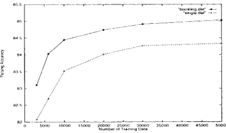
4:.1.2 T h e a m o u n t o f T r a i n i n g D a t a a n d
P a r s i n g A c c u r a c y
Table 6 and Figure 2 show how the n u m b e r of train- ing sentences infhienees parsing accuracy for the same 10000 test sentences. T h e y ilhlstrate the f o r lowing two characteristics of the learning curve.
1. 'file parsing accuracy rapidly rises up to 30000 sentences and converges at a.round 50000 sen- t, enees.
2. T h e maxinlunl parsing accuracy is 84.33% at 50000 training sentences.
We will discuss the n l a x i n m m accuracy of 84.33%. C o m p a r e d to recent stochastic Fnglish parsers t h a t yield 86 to 87(/o accuracy (Collins, 1996; Mager- man, 1995), 84.33% seems unsatisfactory at. the first glance. T h e main reason behind this lies in the dig ference between the two c o r p o r a used: Pelm Tree- bank (Marcus et al., 1993) and E l ) I f corpus (EI)F{,, 1995). l'enn T r e e b a n k ( M a r c u s et M., 1993) was also used to induce part-of-sl)eech (POS) taggers because the corpus contains very precise and det.ailed POS markers as well as bracket annotations. In addition, h;nglish parsers incorporate the. syntactic tags t h a t are contained in the corpns. T h e EDI{ corpus, oil t.he other haud, contains only coarse P O S tags. We used another d apanese POS tagger (M a t s n m o t o and oth- ers, 1996) to make use of well-grained information for disanibiguating syntactic structures. Only the bracket information in the EDI{ corpus was consid- ered. We conjecture t h a t the difference between the parsing accuracies is due to the difference of the cor- pus infonnation. (Fujio and Matsunioto, 1997) con- structed an El)l~-based dependency parser by using a simila.r m e t h o d t.o Collins' (Collins, 19!)6). T h e
parser attained 80.48% accuracy. Although thier
training and Zest. sent.enees are not exactly same as ours, the restllt seems to SUl)port our conjecture on the d a t a difference between E D R and Penn Tree- bank.
4.1.3 S i g n i f i c a n c e o f N o n H e a d - W o r d F e a t u r e s
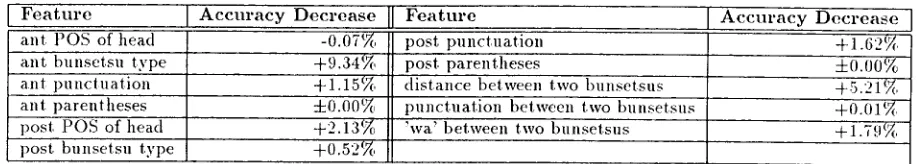
We will now s u m m a r i z e the significance of each non head-word feature introduced in Section 3. The in- fluence of the lexieal information of head words will be discussed in the next section. Table 7 ilhlslrates how the parsing accuracy is reduced when each fea- ture is removed. The m n n b e r of training setttences was 10000. In the table, ant and post. represent the anterior and the posl.erior bnnsetsu, respectiwdy.
Feature ant POS of head ant bunsetsu type ant punctuation ant parentheses post POS of head post bunsetsu type
Accuracy Decrease ][ Feature
-0.07% post punctuation
+9.34% post parentheses
+1.15% distance between two blul.setsus =1=0.00% punctuation between two bunsetsus
+2.13% 'wa' between two bunsetsus
+0.52%
A c c u r a c y Decrease +1.62% +0.00% +5.21% +0.o1% +1.79%
Table 7: Decrease of Parsing Accuracy When Each A t t r i b u t e Removed
H e a d W o r d I n f o r m a t i o n P a r s i n g A c c u r a c y
I 100 words 200 words Level 1 Level 2 ]
83.34% 82.68% 82.51% 81.67%
I
Table 8: Head Word Information v.s. Parsing Accuracy
cant features are anterior bunsetsu type and distance betweell the two bunsetsu. This result m a y partially s u p p o r t an often used heuristic; bunsetsu modifica- tion should be as short range as possible, provided the modification is syntactically possible. In partic- ular, we need to concentrate on the types of bunsetsu to a t t a i n a higher level of accuracy. Most features contribute, to some extent, to the parsing perfor- mance. In our experiment, information on paren- theses has no effect, Oil the performance. T h e reason m a y be t h a t E D R contains only a small n u m b e r of parentheses. One exception in our features is an- t.erior POS of head. We currently hypothesize t h a t this drop of accuracy arises from two reasons.
* In m a u y cases, the POS of head word can be determined from bunsetsu type.
• Our POS tagger sometimes assigns verbs for verb-derived nouns.
4.1.4 Significance of H e a d - w o r d s Lexical I n t b r l n a t i o n
\Ve focused Oil the head-word feature by testing the following 4 lexical sources. The first and the second are the 100 and 200 most frequent words, respec- tively. T h e third and the fourth are derived fl:om a broadly used Japanese thesaurus, Word IAst by Se- mantic Principles (NLRI, 1964). Level 1 and Level 2 classify" words into 15 and 67 categories, respectively.
1. 100 most Frequent words
2. 200 most Frequent words
3. \Vord List. Level 1
4. Word List Level 2
Table 8 displays the parsing accuracy when each head word inforlnation was used in addition to the previous features. The number of training sentences was 10000. In all cases, the performance was worse than 83.52% which was attained without head word lexical information. More surprisingly, more head
word information yielded worse performance. F r o m this result, it. m a y be safely said, at. least for the J a p a n e s e language, t h a t we cannot expect lexical in- forrnation t.o always improve the performance. Fur- ther investigation of other thesaurus and cluster- ing (Charniak, 1997) techniques is necessary to fully understalld the influence of lexical information.
4.2 B o o s t i n g E x p e r i m e n t s
This section reports experimental results on the boosting version of our parser. In all experiments, pruning confidence levels were set. to 55%. Table 9 and Figure 3 show the parsing accuracy when the nulnber of training examples was increased. Because the n u m b e r of iterations in each data set. changed be- tween 5 and 8, we will show the accuracy by combin- ing the first 5 decision trees. In Figure 3, the dotted line plots the learning of the single tree case (identi- cal to Figure 2) for reader's convenience. T h e char- acteristics of the boosting version can be SUlmna- rized as follows c o m p a r e d to the single tree version.
* T h e learning curve rises more rapidly with a small n u m b e r of examples. It is surprising t h a t the boosting version with 10000 sentences per- forms b e t t e r than the single tree version with 50000 sentences.
. T h e boosting version significantly o u t p e r f o r m s the single tree counterpart, for any n u m b e r of sentences although they use the same features for learning.
Next, we discuss how the number of iterations in- fluences the parsing accuracy. Table 10 shows the parsing accuracy for various iteration numbers when 50000 sentences were used as training data. T h e re- suits have two characteristics.
. Parsing accuracy rose up rapidly at the second iteration.
[image:6.612.80.541.47.129.2][ N m n b e r o f T r a i n i n g S e n t e n c e s 3000 6000 10000 20000 30000 50000 ]
P a r s i n g A c c u r a c y 83.10% 84.03% 84.44% 84.74% 84.91% 85.03%
/
Ta.l>le 9: N u m b e r of Training Sentences v.s. Parsing Accuracy
[
N u m b e r o f I t e r a t i o n 1 2 3 4 585.03¢{,
P a r s i n g A c e u r a e y 84.32% 84.93% 84.89% 84.86% ". c,
Table 10: N u m b e r of Iteration v.s. Parsing Accuracy
5
C o n c l u s i o n
We have described a new J a p a n e s e dependency parser t h a t uses decision trc~,s. First, we introduced the single tree parser to clarify the basic character- istics of our method. T h e experimental results show that it. o u t p e r f o r m s conventional stochastic parsers by 4%. Next, the boosting version of our parser w~s introduced, rFhe promising results of the boosting parser can be smmnarized as follows.
• T h e boosting version o u t p e r f o r m s the single- tree c o u n t e r p a r t regardless of training d a t a
a n l o l l n t .
* No data over-titling was seen when the n u m b e r of iterations changed.
We now plan to contitme otlr research ill two direc- tions. One is to make our parser available to a broad range of researchers and to use their feedback to re- vise the features for learning. Second, we will apply our m e t h o d to other languages, say English. Al- though we have focused on the J a p a n e s e language, it is st.raightforward to modify our parser to work with other languages.
8 5
8 4 b
8 1
8 3 5
8 3
8 2 5
8 2
- b ~ o s t . , O a m "
" . . , { l i e d . ~ " - . . . .
+ +
. . . . - . . .
// + ...
, "
5 O O 0 i 0 0 0 0 1 5 0 : 3 0 2 0 o 0 0 250¢K} 3 0 ( ! . 3 0 3 5 0 { i 0 4 0 0 0 ~ . 1 5 0 0 0 5 0 0 0 0 N u m b e r e l qr , a i n l t , g t ) a m
Proc. 15th National Conference on Artificial h+-
lelligcnce, pages 598 603.
Michael Collins. 1996. A New Statistical Parser
based on bigram lexical dependencies. In Proc.
34th Annual Meeling of Association for Compu-
tational Linguistics, pages 184-191.
J a p a n Electronic I)ictionary Reseaech Institute Ltd.
EDR, 1995. 1he EDR Electlvnic Dictionary Tech-
nical Guide.
Yoav Freund and l~obert Schapire. 1996. A
decision-theoretic generalization of on-line learn- ing and an application to boosting.
M. Fujio and Y. M a t s u m o t o . 1997. J a p a n e s e de- pendency s t r u c t u r e analysis based on statistics.
In SIGNL NLI17-12, pages 83-90. (in Jal)anese ).
David M. Magerman. 1995. Statistical Decision-
Tree Models for Parsing. In Proe.3(h'd Annual
Meeting of AssociatioT+ for Compulational Lin-
guistics, pages 276-283.
Mitchell Marcus, Beatrice Santorini, and Mary Ann Marcinkiewicz. 1993. Buihling a large mmot.ated corpus of English: T h e Penn Treebald{. Compu-
lalional Linguistics, 19(2):313 330, June.
Y. M a t s u m o t o el al. 1996. J a p a n e s e Morphological Analyzer Chasen2.0 User's Manual.
NLRI. 1964. Word List by S~manlie Principles.
Syuei Syuppml. (in Japanese).
J.Ross Quinlan. 1993. C/+.5 Programs for Machine
Learning. Morgan Kauflnann Publishers.
Figure 3: l,earning C.urve of Boost.itlg Parser
R e f e r e n c e s
l';ugen( - Charniak. 1993. Slalislical Language Learn- in(I. T h e M I T Press.
[image:7.612.68.291.455.587.2]