Backward Beam Search Algorithm for Dependency Analysis of Japanese

(1)

Backward Beam Search Algorithm

for Dependency Analysis of Japanese

Satoshi Sekine

Computer Science Department New York University 715 Broadway, 7th floor New York, NY 10003, USA

[email protected]

Kiyotaka Uchimoto Hitoshi Isahara

Communications Research Laboratory 588-2 Iwaoka, Iwaoka-cho, Nishi-ku,

Kobe, Hyogo, 651-2492, Japan [uchimoto,isahara]@crl.go.jp

Abstract

Backward beam search for dependency analy-sis of Japanese is proposed. As dependencies normally go from left to right in Japanese, it is effective to analyze sentences backwards (from right to left). The analysis is based on a statisti-cal method and employs a beam search strategy. Based on experiments varying the beam search width, we found that the accuracy is not sen-sitive to the beam width and even the analysis with a beam width of 1 gets almost the same de-pendency accuracy as the best accuracy using a wider beam width. This suggested a determin-istic algorithm for backwards Japanese depen-dency analysis, although still the beam search is effective as the N-best sentence accuracy is quite high. The time of analysis is observed to be quadratic in the sentence length.

1 Introduction

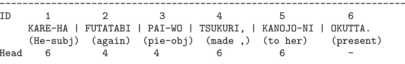
Dependency analysis is regarded as one of the standard methods of Japanese syntactic anal-ysis. The Japanese dependency structure is usually represented by the relationship between phrasal units called ‘bunsetsu’. A bunsetsu usu-ally contains one or more content words, like a noun, verb or adjective, and zero or more func-tion words, like a postposifunc-tion (case marker) or verb/noun suffix. The relation between two bunsetsu has a direction from a dependent to its head. Figure 1 shows examples of bunsetsu and dependencies. Each bunsetsu is separated by “|”. The first segment “KARE-HA” consists of two words, KARE (He) and HA (subject case marker). The numbers in the “head” line show the head ID of the corresponding bunsetsus. Note that the last segment does not have a head, and it is the head bunsetsu of the sentence. The task of the Japanese dependency analysis is to find the head ID for each bunsetsu.

The analysis proposed in this paper has two conceptual steps. In the first step, dependency likelihoods are calculated for all possible pairs of bunsetsus. In the second step, an optimal de-pendency set for the entire sentence is retrieved. In this paper, we will mainly discuss the second step, a method for finding an optimal depen-dency set. In practice, the method proposed in this paper should be able to be combined with any systems which calculate dependency likeli-hoods.

It is said that Japanese dependencies have the following characteristics1:

(1) Dependencies are directed from left to right

(2) Dependencies don’t cross

(3) Each segment except the rightmost one has only one head

(4) In many cases, the left context is not nec-essary to determine a dependency

The analysis method proposed in this paper as-sumed these characteristics and is designed to utilize them. Based on these assumptions, we can analyze a sentence backwards (from right to left) in an efficient manner. There are two merits to this approach. Assume that we are analyzing the M-th segment of a sentence of length N and analysis has already been done for the (M+ 1)-th toN-th segments (M < N). The first merit is that the head of the depen-dency of the M-th segment is one of the

seg-1_{Of course, there are several exceptions (S.Shirai,}

(2)

---ID 1 2 3 4 5 6

Head 6 4 4 6 6

-Translation: He made a pie again and presented it to her.

---Figure 1: Example a Japanese sentence, bunsetsus and dependencies

ments between M + 1 and N (because of as-sumption 1), which are already analyzed. Be-cause of this, we don’t have to keep a huge num-ber of possible analyses, i.e. we can avoid some-thing like active edges in a chart parser, or mak-ing parallel stacks in GLR parsmak-ing, as we can make a decision at this time. Also, we can use the beam search mechanism, by keeping only a certain number of analysis candidates at each segment. The width of the beam search can be easily tuned and the memory size of the pro-cess is proportional to the product of the input sentence length and the beam search width.

The other merit is that the possible heads of the dependency can be narrowed down be-cause of the assumption of non-crossing depen-dencies (assumption 2). For example, if the K-th segment depends on the L-th segment (M < K < L), then the M-th segment can’t depend on any segments between K and L. According to our experiment, this reduced the number of heads to consider to less than 50%.

The technique of backward analysis of Japanese sentences has been used in rule-based methods, for example (Fujita, 1988). How-ever, there are several difficulties with rule-based methods. First the rules are created by humans, so it is difficult to have wide cover-age and keep consistency of the rules. Also, it is difficult to incorporate a scoring scheme in rule-based methods. Many such methods used heuristics to make deterministic decisions (and backtracking if it fails in a searching) rather than using a scoring scheme. However, the com-bination of the backward analysis and the sta-tistical method has very strong advantages, one of which is the beam search.

2 Statistic framework

(3)

3 Algorithm

In this section, the analysis algorithm will be de-scribed. First the algorithm will be illustrated using an example, then the algorithm will be formally described. The main characteristics of the algorithm are the backward analysis and the beam search.

The sentence “KARE-HA FUTATABI PAI-WO TSUKURI, KANOJO-NI OKUTTA. (He made a pie again and presented it to her)” is used as an in-put. We assume the POS tagging and segmen-tation analysis have been done correctly before starting the process. The border of each seg-ment is shown by “|”. In the figures, the head of the dependency for each segment is represented by the segment number shown at the top of each segment.

---<Initial>

ID 1 2 3 4 5 6

---Algorithm

1. Analyze up to the second segment from the end

The last segment has no dependency, so we don’t have to analyze it. The second seg-ment from the end always depends on the last segment. So the result up to the sec-ond segment from the end looks like the following.

---<Up to the second segment from the end>

ID 1 2 3 4 5 6

Cand 6

-

---2. The third segment from the end

This segment (“TSUKURI,”) has two depen-dency candidates. One is the 5th segment (“KANOJO-NI”) and the other is the 6th seg-ment (“OKUTTA”). Now, we use the proba-bilities calculated using the ME model in order to assign probabilities to the two can-didates (Cand1 and Cand2 in the following figure). Let’s assume the probabilities 0.1 and 0.9 respectively as an example. At the tail of each analysis, the total probability (the product of the probabilities of all de-pendencies) is shown. The candidates are sorted by the total probability.

---<Up to the third segment from the end>

ID 1 2 3 4 5 6

Cand1 6 6 - (0.9)

Cand2 5 6 - (0.1)

---3. The fourth segment from the end

For each of the two candidates created at the previous stage, the dependencies of the fourth segment from the end (“PAI-WO”) will be analyzed. For Cand1, the segment can’t have a dependency to the fifth seg-ment (“KANOJO-NI”), because of the non-crossing assumption. So the probabili-ties of the dependencies only to the fourth (Cand1-1) and the sixth (Cand1-2) seg-ments are calculated. In the example, these probabilities are assumed to be 0.6 and 0.4. A similar analysis is conducted for Cand2 (here probabilities are assumed to be 0.5, 0.1 and 0.4) and three candidates are cre-ated (Cand2-1,Cand2-2 and Cand2-3).

---<Up to the fourth segment from the end>

ID 1 2 3 4 5 6

(4)

4. Up to the first segment

The analyses are conducted in the same way up to the first segment. For example, the result of the analysis for the entire sen-tence will be shown below. (Appropriate probabilities are used.)

---<Up to the first segment>

ID 1 2 3 4 5 6

Cand1 6 4 4 6 6 - (0.11) Cand2 4 4 6 6 6 - (0.09) Cand3 6 4 6 5 6 - (0.05)

---Now, the formal algorithm is described induc-tively in Figure 3. The order of the analysis is quadratic in the length of the sentence.

4 Experiments

In this section, experiments and evaluations will be reported. We use the Kyoto University Cor-pus (version 2) (Kurohashi et.al, 1997), a hand created Japanese corpus with POS-tags, bun-setsu segments and dependency information. The sentences in the articles from January 1, 1994 to January 8, 1994 (7,960 sentences) are used for the training of the ME model, and the sentences in the articles of January 9, 1994 (1,246 sentences) are used for the evaluation. The sentences in the articles of January 10, 1994 are kept for future evaluations.

4.1 Basic Result

The evaluation result of our system is shown in Table 1. The experiment uses the correctly seg-mented and part-of-speech tagged sentences of the Kyoto University corpus. The beam search width is set to 1, in other words, the system runs deterministically. Here, ‘dependency accuracy’

Table 1: Evaluation

Dependency accuracy 87.14% (9814/11263) Sentence accuracy 40.60% (503/1239) Average analysis time 0.03 sec

is the percentage of correctly analyzed depen-dencies out of all dependepen-dencies. ‘Sentence accu-racy’ is the percentage of the sentences in which all the dependencies are analyzed correctly.

4.2 Beam search width and accuracy

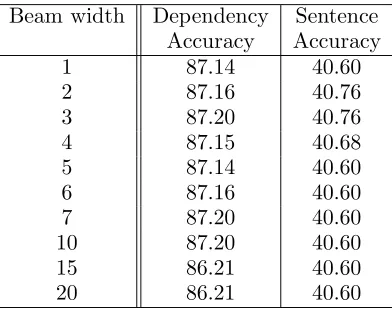
In this subsection, the relationship between the beam width and the accuracy is discussed. In principle, the wider the beam search width, the more analyses can be retained and the better the accuracy can be expected. However, the re-sult is somewhat different from the expectation. Table 2 shows the dependency accuracy and sentence accuracy for beam widths 1 through 20. The difference is very small, but the best

Table 2: Relationship between beam width and accuracy

Beam width Dependency Sentence Accuracy Accuracy

1 87.14 40.60

2 87.16 40.76

3 87.20 40.76

4 87.15 40.68

5 87.14 40.60

6 87.16 40.60

7 87.20 40.60

10 87.20 40.60

15 86.21 40.60

20 86.21 40.60

accuracy is obtained when the beam width is 11 (for the dependency accuracy), and 2 and 3 (for the sentence accuracy). This proves that there are cases where the analysis with the highest product of probabilities is not correct, but the analysis decided at each stage is correct. This is a very interesting result of our experiment, and it is related to assumption 4 regarding Japanese dependency, mentioned earlier.

(5)

---<Variable>

Length: Length of the input sentence in segments W: The beam search width

C[len]: Candidate list; C for each segment keeps the top W partial analyses from that segment to the last segment.

The second segment from the end depends on the last segment. This analysis is stored in C[Length-1].

Assume the analysis up to the (M+1)-th segment has been finished. For each candidate ‘c’ in C[M+1], do the following operation.

Compute the possible dependencies of the M-th segment compatible with ‘c’. For each dependency, create a new candidate ‘d’ by adding the dependency to ‘c’. Calculate the probability of ‘d’. If C[M] has fewer than W entries, add ‘d’ to C[M];

else if the probability of ‘d’ > the probability of the least probable entry of C[M], replace this entry by ‘d’;

else ignore ‘d’.

When the operation finishes for all candidates in C[M+1], proceed to the analysis of the (M-1)-th segment.

Repeat the operation until the first segment is analyzed. The best analysis for the sentence is the best candidate in C[1].

---Figure 2: Formal Algorithm

with the highest probability at each stage also has the highest probability as a whole. This is related to assumption 4. The best analysis with the left context and the best analysis without the left context are the same 95% of the time in general, and 99% of the time if the analysis is correct. These numbers are much higher than our human experiment mentioned in the ear-lier footnote (note that the number here is the percentage in terms of sentences, and the num-ber in the footnote is the percentage in terms of segments.) It means that we may get good ac-curacy even without left contexts in analyzing

Japanese dependencies.

4.3 N-Best accuracy

(6)

Table 3: The rank of the deterministic analysis

80 Sentence Accuracy

*

Figure 3: N-best sentence Accuracy

an ideal system for finding the correct analysis among them, which may use semantic or con-text information, we can have a very accurate analyzer.

We can make two interesting observations from the result. The accuracy of the 1-best analysis is about 40%, which is more than half of the accuracy of 20-best analysis. This shows that although the system is not perfect, the computation of the probabilities is probably good in order to find the correct analysis at the top rank.

The other point is that the accuracy is sat-urated at around 80%. Improvement over 80% seems very difficult even if we use a very large beam width W. (If we set W to the number of all possible combinations, which means al-mostL! for sentence lengthL, we can get 100% N-best accuracy, but this is not worth consider-ing.) This suggests that we have missed some-thing important. In particular, from our inves-tigation of the result, we believe that coordinate

structure is one of the most important factors to improve the accuracy. This remains one area of future work.

4.4 Speed of the analysis

Based on the formal algorithm, the analysis time can be estimated as proportional to the square of the input sentence length. Figure 4 shows the relationship between the analysis time and the sentence length when we set the beam width to 1. We use a Sun Ultra10 ma-chine and the process size is about 8M byte. We can see that the actual analyzing time

al-0 10 20 30 40

Sentence length 0

0.1 0.2 0.3

Analysis time (sec.)

*

Figure 4: Relationship between sentence length and analyzing time

(7)

5 Conclusion

In this paper, we proposed a statistical Japanese dependency analysis method which processes a sentence backwards. As dependencies normally go from left to right in Japanese, it is effective to analyze sentences backwards (from right to left). In this paper, we proposed a Japanese de-pendency analysis which combines a backward analysis and a statistical method. It can nat-urally incorporate a beam search strategy, an effective way of limiting the search space in the backward analysis. We observed that the best performances were achieved when the width is very small. Actually, 95% of the analyses ob-tained with beam width=1 were the same as the best analyses with beam width=20. The analysis time was proportional to the square of the sentence length (number of segments), as was predicted from the algorithm. The average analysis time was 0.03 second (average sentence length was 10.0 bunsetsus) and it took 0.29 sec-ond to analyze the longest sentence, which has 41 segments. This method can be applied to various languages which have the same or simi-lar characteristics of dependencies, for example Koran, Turkish etc.

References

Adam Berger and Harry Printz. 1998 : “A Comparison of Criteria for Maximum En-tropy / Minimum Divergence Feature Selec-tion”. Proceedings of the EMNLP-98 97-106 Michael Collins. 1997 : “Three Generative,

Lexicalized Models for Statistical Parsing”.

Proceedings of the ACL-97 16-23

Terumasa Ehara. 1998 : “Calculation of Japanese dependency likelihood based on Maximum Entropy model”. Proceedings of

the ANLP, Japan 382-385

Masakazu Fujio and Yuuji Matsumoto. 1998 : “Japanese Dependency Structure Analysis based on Lexicalized Statistics”. Proceedings

of the EMNLP-98 87-96

Katsuhiko Fujita. 1988 : “A Trial of determin-istic dependency analysis”. Proceedings of the Japanese Artificial Intelligence Annual meet-ing 399-402

Masahiko Haruno and Satoshi Shirai and Yoshi-fumi Ooyama. 1998 : “Using Decision Trees to Construct a Practical Parser”. Proceedings

of the the COLING/ACL-98 505-511

Sadao Kurohashi and Makoto Nagao. 1994 : “KN Parser : Japanese Dependency/Case Structure Analyzer”. Proceedings of The In-ternational Workshop on Sharable Natural

Language Resources 48-55

Sadao Kurohashi and Makoto Nagao. 1997 : “Kyoto University text corpus project”. Pro-ceedings of the ANLP, Japan 115-118

David Magerman. 1995 : “Statistical Decision-Tree Models for Parsing”. Proceedings of the

ACL-95 276-283

Adwait Ratnaparkhi. 1997 : “A Linear Ob-served Time Statistical Parser Based on Maximum Entropy Models”. Proceedings of EMNLP-97

Satoshi Sekine and Ralph Grishman. 1995 : “A Corpus-based Probabilistic Grammar with Only Two Non-terminals”. Proceedings of the

IWPT-95 216-223

Satoshi Shirai. 1998 : “Heuristics and its lim-itation”. Journal of the ANLP, Japan Vol.5 No.1, 1-2

Kiyoaki Shirai, Kentaro Inui, Takenobu Toku-naga and Hozumi Tanaka. 1998 : “An Em-pirical Evaluation on Statistical Parsing of Japanese Sentences Using Lexical Association Statistics”. Proceedings of EMNLP-98 80-86 Kiyotaka Uchimoto, Satoshi Sekine, Hitoshi Isahara. 1999 : “Japanese Dependency Structure Analysis Based on Maximum En-tropy Models”. Proceedings of the EACL-99