Grammar induction from (lots of) words alone

Grammar induction from (lots of) words alone

John K Pate

Department of Linguistics The University at Buffalo Buffalo, NY 14260, USA johnpate@buffalo.edu

Mark Johnson

Department of Computing Macquarie University Sydney, NSW 2109, Australia mark.johnson@mq.edu.au

Abstract

Grammar induction is the task of learning syntactic structure in a setting where that structure is hidden. Grammar induction from words alone is interesting because it is similiar to the problem that a child learning a language faces. Previous work has typically assumed richer but cognitively implausible input, such as POS tag annotated data, which makes that work less relevant to human language acquisition. We show that grammar induction from words alone is in fact feasible when the model is provided with sufficient training data, and present two new streaming or mini-batch algorithms for PCFG inference that can learn from millions of words of training data. We compare the performance of these algorithms to a batch algorithm that learns from less data. The minibatch algorithms outperform the batch algorithm, showing that cheap inference with more data is better than intensive inference with less data. Additionally, we show that the harmonic initialiser, which previous work identified as essential when learning from small POS-tag annotated corpora (Klein and Manning, 2004), is not superior to a uniform initialisation.

1 Introduction

How children acquire the syntax of the languages they ultimately speak is a deep scientific question of fundamental importance to linguistics and cognitive science (Chomsky, 1986). The natural language pro-cessing task of grammar induction in principle should provide models for how children do this. However, previous work on grammar induction has learned from small datasets, and has dealt with the resulting data sparsity by modifying the input and using careful search heuristics. While these techniques are use-ful from an engineering perspective, they make the models less relevant to human language acquisition.

In this paper, we use scalable algorithms for Probabilistic Context Free Grammar (PCFG) inference to perform grammar induction from millions of words of speech transcripts, and show that grammar induction from words alone is both feasible and insensitive to initialization. To ensure the robustness of our results, we use two algorithms for Variational Bayesian PCFG inference, and adapt two algorithms that have been proposed for Latent Dirichlet Allocation (LDA) topic models. Most importantly, we find that the three algorithms that scale to large datasets improve steadily over training to about the same predictive probability and parsing performance.

Moreover, while grammar induction from small datasets of POS-tagged newswire text fails without careful ‘harmonic’ initialization, we find that initialization is much less important when learning directly from larger datasets consisting of words alone. Of the algorithms in this paper, one does 2.5% better with harmonic initialization, another does 5% worse, and the other two are insensitive to initialization.

The rest of the paper is organized as follows. In Section 2, we discuss previous grammar induction research, in Section 3 we present the particular model grammar we will use, in Section 4 we describe the inference algorithms, and in Section 5 we present our experimental results.

This work is licenced under a Creative Commons Attribution 4.0 International License. License details: http:// creativecommons.org/licenses/by/4.0/

2 Background

Previous grammar induction work has used datasets with at most 50,000sentences. Fully-lexicalized models would struggle with data sparsity on such small datasets, so previous work has assumed input in either the form of part-of-speech (POS) tags (Klein and Manning, 2004; Headden III et al., 2009) or word representations trained on a large external corpus (Spitkovsky et al., 2011; Le and Zuidema, 2015). Some previous work has moved towards learning from word strings directly. Bisk and Hockenmaier (2013) used combinatory categorial grammar (CCG) to learn syntactic dependencies from word strings. However, they initialise their model by annotating nouns, verbs, and conjunctions in the training set with atomic CCG categories using a dictionary, and so do not learn from words alone. Pate and Goldwater (2013) learned syntactic dependencies from word strings alone, but used sentences from the Switchboard corpus of telephone speech that had been selected for prosodic annotation and so were unusually fluent. Kim and Mooney (2010), B¨orschinger et al. (2011), and Kwiatkowski et al. (2012), learned from word strings together with logical form representations of sentence meanings. While children have situational cues to sentence meaning, these cues are ambiguous, and it is difficult to represent these cues in a way that is not biased towards the actual sentences under consideration. We focus on the evidence for syntactic structure that can be obtained from word strings themselves.

Grammar induction directly from word strings is interesting for two reasons. First, this problem setting more closely matches the language acquisition task faced by an infant, who will not have access to POS tags or a corpus external to her experience. Second, this setting allows us to attribute behavior of grammar induction systems to the underlying model itself, rather than additional annotations made to the input. Approaches to grammar induction that involve replacing words with POS tags or other lexical or syntactic observed labels make the process significantly more difficult to understand or compare across genres or languages, as the results will depend on exactly how these labels are assigned. Models that only require words alone as input do not suffer from this weakness.

3 PCFGs and the Dependency Model with Valence

3.1 Probabilistic Context Free Grammars

A Probabilistic Context Free Grammar is a tuple(W,N, S,R,θ), whereW andN are sets of terminal and non-terminal symbols,S ∈ N is a distinguished start symbol, andRis a set of production rules. θ is a vector of multinomial parameters of length|R|indexed by production rulesA → β, soθA→β

is the probability of the productionA → β. We useRAto denote all rules with left-hand sideA, and

useθAto denote the subvector ofθ indexed by the rules inRA. We require for all rules,θA→β ≥ 0,

and for allA∈N,P_A→β∈R_AθA→β = 1, and use∆to denote the probability simplex satisfying these

constraints. The yieldy(t)of a tree tis the string of terminals oft, and the yield of a vector of trees T = (t1, . . . , t|T|)is the vector of yields of each tree: y(T) = (y(t1), . . . ,y(t|T|)). The probability of

generating a treetgiven parametersθis:

PG(t|θ) = Y

A→β∈R

θf(t,A→β) r

wheref(t, A→β)is the number of times ruleA→β is used in the derivation oft.

To model uncertainty in the parameters, we draw the parameters of each multinomial θA from a

prior distributionP(θA|αA), where the vector of hyperparametersαA defines the shape of this prior

distribution (and αis just the concatenation of eachαA). The joint probability of a vector of treesT

with one treeti for each sentencesi, and parametersθis then:

P(T,θ|α) =P(T|θ)P(θ|α) = Y A→β∈R

θf(T,A→β) A→β

" Y

A∈N

P(θA|αA) #

Dirichlet priors for these multinomials are both standard and convenient:

PD(θA|αA) =

ΓP_A→β∈R_AαA→β Q

A→β∈RAΓ(αA→β)

Y

A→β∈RA

θαA→β−1

A→β

where the Gamma functionΓgeneralizes the factorial function from integers to real numbers. Dirichlet distributions are convenient priors because they areconjugateto multinomial distributions: the product of a Dirichlet distribution and a multinomial distribution is itself a Dirichlet distribution:

P(T,θ|α) =PG(T|θ)PD(θ|α)∝ Y

A→β∈R

θf(T,A→β)+α_A→β−1

A→β (1)

For grammar induction, we observe only the corpus of sentences C, and modify Equation 1 to marginalize over trees and rule probabilities.

P(C|α) = X T:y(T)=C

Z

∆P(T,θ|α)dθ (2)

This sum over trees introduces dependencies that make exact inference intractable.

We assessed grammar induction from words alone using the Dependency Model with Valence (DMV) (Klein and Manning, 2004). In the original presentation, it first draws the root of the sentence from aProot

distribution over words, and then generates the dependents of headhin each directiondir ∈ {←,→} in a recursive two-step process. First, it decides whether to stop generating (a Stop decision) according toPstop(·|h,dir, v), wherev indicates whether or noth has any dependents in the direction ofdir. If

it does not stop (a¬Stop decision), it draws the dependent worddfromPchoose(d|h,dir). Generation ceases when all words stop in both directions.

Johnson (2007) and Headden III et al. (2009) reformulated this generative process as a split-head bilexical PCFG (Eisner and Satta, 2001) so that the rule probabilities are DMV parameters. Such a PCFG represents each token of the string with two ‘directed’ terminals that handle leftward and rightward decisions independently, and defines rules and non-terminal symbols schematically in terms of terminals. Minimally, we need rightward-lookingRw, leftward-lookingLw, and undirectedYwnon-terminal labels

for each word w. The grammar has a rule for each dependent worddof a head wordh from the left (Lh → Yd Lh) and from the right (Rh → Rh Yd), a rule for each a wordwto be the sentence root

(S → Yw), and a rule for each undirected symbol to split into directed symbols (Yw → Lw Rw).

To incorporate Stop decisions into the grammar, we distinguished non-terminals that dominate a Stop decision from those that dominate a Choose decision by decorating Choose non-terminals with 0 _{(so a}

left attachment rule isL0

h → Yd Lh), and introduced unary rules that rewrite to terminals (Lh →hl) for

Stop decisions, and to Choose non-terminals (Lh → L0_h) for¬Stop decisions. We implemented valence

with a superscript decoration on each non-terminal label: L0

h indicateshhas no dependents to the left,

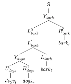
andLh indicates that h has at least one dependent to the left. Figure 1 presents PCFG rule schemas

with their DMV parameters, and dependency and split-head PCFG trees for “dogs bark.” We use several inference algorithms to learn production weights for this PCFG, and study how the parsing accuracy varies with algorithm and computational effort.

4 Inference1

One central challenge of learning from words alone is data sparsity. Data sparsity is most naturally addressed by learning from large amounts of data, which is easily available when learning from words alone, so we use algorithms that scale to large datasets. To ensure that our system reflects the underlying relationship between the model and the data, we explore three such algorithms. These algorithms are ex-tensions of the batch algorithm for variational Bayesian (batch VB) inference of PCFGs due to Kurihara

PCFG Rule DMV parameter S → Yh Proot(h)

Yh → L0h R0h 1

L0

h → hl Pstop(Stop|h,←,no dep)

L0

h → L

0

h Pstop(¬Stop|h,←,no dep)

L0_h → Yd Lh Pchoose(d|h,←)

Lh → hl Pstop(Stop|h,←,one dep)

Lh → L0h Pstop(¬Stop|h,←,one dep)

(a) Split-head rule schemas and corresponding probabilities for the DMV. The rules expandingL0

h and Lh symbols encode

Stop decisions with no dependents and at least one dependent, respectively, and the the rules expandingL0

hsymbols encode

Choose decisions.

S Ybark

L0 bark

L0_bark

Ydogs

L0 dogs

dogs_l

R0 dogs

dogs_r

Lbark

barkl

R0 bark

barkr

(b) Tree for “dogs bark” using the grammar in Figure 1a.

dogs bark ROOT

(c) Example dependency tree with one root and left arc.

Figure 1: The DMV as a PCFG, and dependency and split-head bilexical CFG trees for “dogs bark.”

and Sato (2004), so we first review batch VB. Inspired by the reduction of LDA inference to PCFG in-ference presented in Johnson (2010), we then develop new streaming on-line PCFG inin-ference algorithms by generalising the streaming VB (Broderick et al., 2013) and stochastic VB (Hoffman et al., 2010) al-gorithms for Latent Dirichlet Allocation (LDA) to PCFG inference. We finally review the collapsed VB algorithm due to Wang and Blunsom (2013) for PCFGs that we compare to the other algorithms.

Figure 2 summarizes the four algorithms for PCFG inference. 4.1 Batch VB

Kurihara and Sato’s (2004) batch algorithm for variational Bayesian inference approximates the pos-terior P(T,θ|C,α)by maximizing a lower bound on the log marginal likelihood of the observations

lnP(C|α). This lower boundLinvolves a variational distributionQ(T,θ)over unobserved variables T andθ. By Jensen’s inequality, for any distributionQ(T,θ), we have:

lnP(C|α) = lnX T

Z

Q(T,θ)P(C,_Q(TT_,,_θθ₎|α)dθ≥X

T Z

Q(T,θ) lnP(C,_Q(TT_,,_θθ₎|α)dθ =L

lnP(C|α)− Lis the Kullback-Leibler divergence KL(Q(T,θ)||P(T,θ|C,α)). Variational inference adjusts the parameters of the variational distribution to maximizeL, which minimizes the KL divergence. VB makes inference tractable by factorizing the variational posterior. The mean-field factorization assumes parameters and trees are independent: Q(T,θ) = Qθ(θ)

Q_|T|

i=1QT(ti). Kurihara and Sato

showed thatQθ(θ)is also a product of Dirichlet distributions, whose hyperparametersαˆAare a sum of

the prior hyperparametersαA→βand the expected count ofA→βacross the corpus underQT:

ˆ

αA→β =αA→β + |C| X

i=1 ˆ

f(si, A→β)

ˆ

f(s, A→β) =EQT[f(t, A→β)]

f(t, A→β)is the number of times ruleA→ β is used in the derivation of treet. fˆ(si, A→β)is the

expected number of timesA→βis used in the derivation of sentencesi, and can be computed using the

expected counts, andQT, using the hyperparametersαˆ ofQθ to compute probability-like ratiosπA→β:

QT(t) = Y

A→β∈R

πf_A(_→t,A_β→β) πA→β = exp (Ψ (ˆαA→β)) expΨP_A→β0_∈R

AαˆA→β0

where the digamma functionΨ(·)is the derivative of the log Gamma function. Algorithm 1 presents the full algorithm.

4.2 Scalable VB algorithms

Batch VB requires a complete parse of the training data before parameter updates, which is computation-ally intensive. We explore three algorithms that divide the data into minibatchesC =C(1)_{, . . . ,C}(n)

and update parameters after parsing each minibatch.

Streaming VB: Broderick et al. (2013) proposed a ‘streaming VB’ algorithm for LDA that approxi-mates Bayesian Belief Updates (BBU) to make a single pass through the training data. A BBU uses the current posterior as a prior to compute the next posterior without reanalyzing previous minibatches:

Pθ|C(1), . . . ,C(n)∝PC(n)|θPθ|C(1), . . . ,C(n−1)

However, the normalization constant involves an intractable marginalization. Broderick et al. suggested approximating each posterior with some algorithmAthat computes an approximate posteriorQ(n)_given

a minibatchC(n)_{and the previous posteriorQ}(n−1)_:

Pθ|C(1), . . . ,C(n)≈Q(n)(θ) =AC(n), Q(n−1)(θ)

whereQ(0) _{is the true prior. By using a mean-field VB algorithm for LDA inference forA, they}

ap-proximate each subsequentQ(n)_{as a product of Dirichlets, whose hyperparameters are a running sum of}

expected counts from previous minibatches and prior hyperparameters. We used the batch VB algorithm forAto generalise this algorithm to PCFG inference. Algorithm 2 presents the full algorithm.

Stochastic VB: Hoffman et al. (2010) proposed a ‘stochastic VB’ algorithm for LDA that uses each minibatch to compute the maximum of an estimate of the natural gradient of L. This maximum is obtained by computing expected counts forC(i)_{, and scaling the counts as though they were gathered}

from the full dataset. The new hyperparameters are obtained by taking a step toward the maximum: α(_Aen_→+_βi) = (1−η)α(_Aen_→+_βi−1)+ηl(_Ai)_→βfˆ(en+i)(A→β)

whereηis the step size,fˆ(en+i)_{(A→β)is the expected count of ruleA → βin minibatchiof epoch}

e, andl(_Ai)_→β is the scaling term for ruleA → β. In their LDA inference procedure, each word has one topic, so the scaling term is the number of words in the full dataset divided by the number of words in the minibatch. For the DMV, a string swith |s|terminals has one root, |s| −1choose rules, and

2|s|+ (|s| −1)stop decisions (two Stops and one¬Stop rule for each arc). The scaling terms are then: root rules choose rules stop rules

l(_Si_→) _Yh = |C|

|C(i)| l (i) A→β =

P|C|

j=1|sj|−1

P|C(i)|

j0=1 |sj0|−1

l_A(i)_→β = Pj=1|C| 2|sj|+|sj|−1

P|C(i)|

j0=1 2|sj0|+|sj0|−1

Collapsed VB: Teh et al. (2007) proposed, and Asuncion et al. (2009) simplified, a ‘collapsed VB’ algorithm for LDA that integrates out model parameters and so achieves a tighter lower bound on the marginal likelihood. This algorithm cycled through the training set and optimized variational distribu-tions over the topic assignment of each word given all the other words.

Wang and Blunsom (2013) generalized this algorithm to PCFGs. The variational distribution for each sentence is parameterized by expected rule counts for that sentence, and they optimize each sentence-specific distribution by cycling through the corpus and optimizing the distribution over trees for sentence siusing counts from all the other sentencesC(¬i). The exact optimization, marginalizing over rule

Data:a corpus of stringsC

Initialization: prior hyperparametersα

1 αˆ(0)=α

2 forj= 1tomdo

3 π_A→β = exp

Ψαˆ(j_A→−1)_β

exp

Ψ

P

A→β0∈R_Aαˆ(j_A→−1)_β0

4 fori= 1to|C|do 5 fˆ(j)(s_i, A→β) =

Eπ[f(t, A→β)]

6 end

7 αˆ(j)=α+ ˆf(j) 8 end

output:αˆ(m)

Algorithm 1:Batch VB. Here,αˆ(j)_{are the}

pos-terior counts after iterationj, which define rule weightsπfor the next iteration.

Data:nminibatchesC(1)_{, . . . ,C}(n)

Initialization: prior hyperparametersα

1 αˆ(0) =α 2 fori= 1tondo

3 ∀A→β ∈R fˆ(0)(A→β) = 0 4 forj= 1tomdo

5 π_A→β =

exp(Ψ(fˆ(C(i),A→β)+ˆα_A→β))

expΨP

A→β0∈R_Afˆ(C(i),A→β0)+ˆαA→β0

6 fˆ(i,j)(A→β) =Eπ[f(t, A→β)]

7 end

8 αˆ(i)= ˆf(i,m)+ ˆα(i−1) 9 end

output:αˆ(n)

Algorithm 2: Streaming VB with m steps of VB per minibatch. fˆ(j)_{(A→β) is the}

ex-pected count of ruleA→βin theith_minibatch

afterjiterations. Data:nminibatchesC(1)_{, . . . ,C}(n)

Initialization: prior hyperparametersα, step size schedule parameters τ,κ, epoch countE

1 αˆ(0)=α

2 fore= 0toE−1do 3 fori= 1tondo 4 π_A→β =

exp

Ψ

ˆ

α(en+i_A→β−1)

expΨP

A→β0∈R_Aαˆ(en+i_A→β0−1)

5 fˆ(en+i)(A→β) = Eπ[f(t, A→β)]

6 η= (τ+i)−κ 7 forA→β ∈Rdo

8 αˆ(_Aen_→+_βi)= (1−η) ˆα(_Aen_→+_βi−1)+

ηl(_Ai)_→βfˆ(en+i)_(A→β)

9 end

10 end 11 end

output:αˆ(n)

Algorithm 3:Stochastic VB.fˆ(en+i)_(A→β)

is the expected count of rule A→β in the ith

minibatch in theeth_{epoch, andl}(i)

A→βis the

scal-ing parameter for ruleA → β for theith

mini-batch, as described in the text.

Data:nsingle-string minibatches C(1)_{, . . . ,C}(n)

Initialization: prior hyperparametersα, epoch countE, initial sentence-specific expected countsfˆ

1 αˆ =α+Pn_i=1fˆ(i) 2 fore= 0toE−1do 3 fori= 1tondo 4 αˆ = ˆα−fˆ(i)

5 π_A→β = P αˆA→β

A→β0∈R_AαˆA→β0

6 fˆ(i)(A→β) =Eπ[f(t, A→β)]

7 αˆ = ˆα+ ˆf(i) 8 end

9 end

output:sentence-specific expected countsfˆ, global hyperparametersαˆ

Algorithm 4: Collapsed VB. fˆ(i)_{(A→β) is}

the expected count of rule A→β for the ith

sentence, and the global hyperparametersαˆ are the sum of the expected counts for each sen-tence and prior hyperparameters.

train dev test

Swbd

Words 363,902 24,015 23,872 Sentences 43,577 2,951 2,956

Fisher

Words 5,576,173 – –

Sentences 664,346 – – Table 1: Data set sizes. Fisher is only for training.

5 Experiments

We evaluate how millions of words of training data affects grammar induction from words alone by examining learning curves. We ran each algorithm 5 times, each with a different random shuffle of the training data on each run, and evaluated on the test set at logarithmically-spaced numbers of training sentences. Stochastic, collapsed, and batch VB used more than one pass over the training corpus, while streaming VB makes one pass over the training corpus. To obtain a consistent horizontal axis in our learning curves, we plot learning curves as a function of computational effort, which we measure by the number of sentences parsed, since almost all the computational effort of all the algorithms is in parsing. Stochastic, collapsed, and streaming VB can learn from the full training corpus (although collapsed VB requires more RAM – 60GB rather than 6GB for us – as it stores expected rule counts for each sentence). Batch VB required about 50 iterations for convergence for large training sets, and so cannot be applied to the full training set due to long training times. We used batch VB with training sets of up to100,000strings.

5.1 Hyperparameters and initialization

We use Dirichlet priors with symmetric hyperparameter α = 1for all algorithms (preliminary experi-ments showed that the algorithms are generally insensitive to hyper-parameter settings). We ran batch VB until the log probability of the training set changed less than 0.001%. For stochastic VB, we used κ= 0.9,τ = 1, and minibatches of 10,000 sentences. To investigate convergence and overfitting, we ran stochastic and collapsed VB for 15 epochs of random orderings of the training corpus. For streaming VB, the first minibatch had10,000sentences, the rest had1, and we used one iteration of VB per minibatch. Klein and Manning (2004) showed that initialization strongly influences the quality of the induced grammar when training from POS-tagged WSJ10 data, and they proposed a harmonic initialization pro-cedure that puts more weight on rules that involve terminals that frequently appear close to each other in the training data. We present results both for a uniform initialization, where the only counts initially are the uninformative Dirichlet priors (plus, for collapsed VB, random sentence-specific counts), and a harmonic initialization. For streaming VB, harmonic counts are gathered from each minibatch, and for the others, harmonic counts are gathered from the entire training set.

5.2 Data

We present experiments on two corpora of words from spontaneous speech transcripts. Our first corpus is drawn from the Switchboard portion of the Penn Treebank (Calhoun et al., 2010; Marcus et al., 1993). We used the version produced by Honnibal and Johnson (2014), who used the Stanford dependency converter to convert the constituency annotations to dependency annotations (Catherine de Marneffe et al., 2006). We used Honnibal and Johnson’s train/dev/test partition, and ignored their second dev partition. We discarded sentences shorter than four words from all partitions, as they tend to be formulaic backchannel responses (Bell et al., 2009), and sentences with more than 15 words (long sentences did not improve accuracy on the dev set).

Harmonic Init Non-harmonic Init

0.20 0.25 0.30 0.35 0.40

-400000 -350000 -300000

Directed

accurac

y

Log

probability

1e+02 1e+04 1e+06 1e+02 1e+04 1e+06 Computational effort (total number of sentences parsed)

Inference Batch VB Collapsed VB Stochastic VB Streaming VB

Figure 3: Directed accuracy (top) and predictive log probability (bottom) of test-set sentences from Switchboard with 4-15 words. The horizontal axis is the number of sentences parsed (all algorithms except streaming VB re-parse sentences multiple times). The left column presents inference with a harmonic initialization, and the right column presents inference with a uniform initialization (and, for collapsed VB, random sentence-specific counts). The black line is a uniform-branching baseline.

each word type, and5,381,644Choose rules. Table 1 presents data set sizes. 5.3 Evaluation measures

We evaluated all algorithms in terms of predictive log probability and directed attachment accuracy. We computed the log probability of the evaluation set under posterior mean parameters, obtained by normalizing counts. Directed accuracy is the proportion of arcs in the Viterbi parse that match the gold standard, including the root. We also compared with a left-branching baseline, since it outperformed a right-branching baseline. A left-branching (right-branching) baseline sets the last (first) word of each sentence to be the root, and assigns each word to be the head of the word to its left (right). The left-branching baseline on this dataset is about 0.29, while on the traditionalwsj10 dataset of Klein and Manning (2004) it is 0.336, suggesting our dataset, with longer sentences, is somewhat more difficult. 5.4 Results

The bottom row of Figure 3 presents the predictive log probability of the test set under the posterior mean parameter vector as training proceeds. The figure contains one point per evaluation per run, and a loess-smoothed curve for each inference type. We see among all algorithms that the log probability of the test set constantly increases, regardless of initialization, with one exception. The sole exception is streaming VB with harmonic initialization, where predictive log probability drops after the initial minibatch of 10,000 sentences. Streaming VB with harmonic init parses each sentence of the initial minibatch using prior pseudocounts and harmonic counts. We will return to this drop when we discuss accuracy.

the importance of harmonic initialisation reflect the small training data sets used in those experiments. The top row of Figure 3 presents directed accuracy on the test set as training proceeds. As in the pre-dictive probability evaluation, there is no clear advantage to a harmonic initialization across algorithms. Batch VB and collapsed VB perform identically with both initializations, and streaming VB ultimately does 5% better while stochastic VB does 2.5% worse. While streaming VB showed a drop in predictive probability after the initial 10,000 sentence minibatch with harmonic initialization, it obtains a small but sharp improvement in parse accuracy at the same point. These two results suggest that the harmonic initialization, applied to words, captures regularities that are not syntactic but still explain data well.

The inference algorithms differ most obviously when they have parsed few sentences, indicating that each algorithm’s bias is strongest in the face of small data. Streaming VB learns slowly initially because, throughout the large initial minibatch, it gathers counts using only the uninformative prior or only the uninformative prior plus harmonic counts. Collapsed VB, on the other hand, has sentence-specific counts for the entire training corpus even in the random case. These counts provide a rough estimate of how many opportunities there are for an arc to exist between each word in each direction at each valence, and therefore provide a stronger starting point that takes more time to overcome. Finally, the good performance of stochastic VB with small datasets, compared to streaming VB and batch VB, may reflect the conservatism of only taking a step in the direction of the gradient rather than always maximizing.

Regardless of the details of the different algorithms’ performance, we see that they all steadily im-prove or stabilize as inference proceeds over a large dataset, and that initialization is not important when learning from large numbers of words.

6 Conclusion

Grammar induction from words alone has the potential to address important questions about how children learn and represent linguistic structure, but previous work has struggled to learn from words alone in a principled way. Our experiments show that grammar induction from words alone is feasible with a simple and well-known model if the dataset is large enough, and that heuristic initialization is not necessary (and may even interfere). Future computational work on child language acquisition should take advantage of this finding by applying richer models of syntax to large datasets, and learning distributed word representations jointly with syntactic structure.

References

Arthur Asuncion, Max Welling, Padhraic Smyth, and Yee Whye Teh. 2009. On smoothing and inference for topic models. InUncertainty in Artificial Intelligence.

Alan Bell, Jason M Brenier, Michelle Gregory, Cynthia Girand, and Dan Jurafsky. 2009. Predictability effects on durations of content and function words in conversational English. Journal of Memory and Language, 60:92– 111.

Yonatan Bisk and Julia Hockenmaier. 2013. An HDP model for inducing Combinatory Categorial Grammars.

Transactions of the Association for Computational Linguistics, 1(Mar):75–88.

Benjamin B¨orschinger, Bevan K Jones, and Mark Johnson. 2011. Reducing grounded learning tasks to grammat-ical inference. InProceedings of the 2011 conference on Emprical Methods in Natural Language Processing

(EMNLP), pages 1416–1425.

Tamara Broderick, Nicholas Boyd, Andre Wibisono, Ashia C Wilson, and Michale I Jordan. 2013. Streaming variational bayes. InNeural Information Processing Systems.

S Calhoun, J Carletta, J Brenier, N Mayo, D Jurafsky, M Steedman, and D Beaver. 2010. The NXT-format Switchboard corpus: A rich resource for investigating the syntax, semantics, pragmatics and prosody of dia-logue. Language Resources and Evaluation, 44(4):387–419.

Marie Catherine de Marneffe, Bill MacCartney, and Christopher D Manning. 2006. Generating typed dependency parses from phrase structure parses. InProceedings of the 5th International Conference on Language Resources

Noam Chomsky. 1986. Knowledge of language: Its nature, origin, and use.

Jason Eisner and Giorgio Satta. 2001. Efficient parsing for bilexical context-free grammars and head-automaton grammars. InACL.

Will Headden III, Mark Johnson, and David McClosky. 2009. Improved unsupervised dependency parsing with richer contexts and smoothing. InNAACL-HLT.

M Hoffman, D M Blei, and F Bach. 2010. Online learning for latent dirichlet allocation. InProceedings of NIPS. Matthew Honnibal and Mark Johnson. 2014. Joint incremental disfluency detection and dependency parsing.

Transactions of the Association for Computational Linguistics, 2(April):131–142.

Mark Johnson. 2007. Transforming projective bilexical dependency grammars into efficiently-parseable CFGs with unfold-fold. InACL.

Mark Johnson. 2010. PCFGs, topic models, adaptor grammars and learning topical collocations and the structure of proper names. InProceedings of the Association for Computational Linguistics.

Joohyun Kim and Raymond J Mooney. 2010. Generative alignment and semantic parsing for learning from am-biguous supervision. InProceedings of the 23rd international conference on computational linguistics

(COL-ING 2010).

Dan Klein and Christopher D. Manning. 2004. Corpus-based induction of syntactic structure: Models of depen-dency and constituency. InProceedings of ACL, pages 479–486.

Kenichi Kurihara and Taisuke Sato. 2004. An application of the Variational Bayesian approach to probabilistic context-free grammars. InIJCNLP 2004 Workshop beyond Shallow Analyses.

Tom Kwiatkowski, Sharon Goldwater, Luke Zettlemoyer, and Mark Steedman. 2012. A probabilistic model of syntactic and semantic acquisition from child-directed utterances and their meanings. InProceedings of the European Chapter of the Association for Computational Linguistics.

K Lari and S J Young. 1990. The estimation of stochastic context-free grammars using the inside-outside algo-rithm. Computer Speech and Language, 5:237–257.

Phong Le and Willem Zuidema. 2015. Unsupervised dependency parsing: Let’s use supervised parsers. In

Proceedings of ACL.

Mitchell P Marcus, Beatrice Santorini, and Mary Ann Marcinkiewicz. 1993. Building a large annotated corpus of English: The Penn Treebank. Computational Linguistics, 19(2):313–330.

John K Pate and Sharon Goldwater. 2013. Unsupervised dependency parsing with acoustic cues. Transactions of the ACL.

Valentin I Spitkovsky, Hiyan Alshawi, Angel X Chang, and Daniel Jurafsky. 2011. Unsupervised dependency parsing without gold part-of-speech tags. In Proceedings of the 2011 Conference on Empirical Methods in

Natural Language Processing (EMNLP 2011).

Yee Whye Teh, David Newman, and Max Welling. 2007. A collapsed variational Bayesian inference algorithm for latent Dirichlet allocation. InNeural Information Processing Systems, volume 19, pages 705–729.

Pengyu Wang and Phil Blunsom. 2013. Collapsed variational bayesian inference for PCFGs. InProceedings the