Article
Retrieval of Non-Optically Active Parameters for
Small Scale Urban Waterbodies by a Machine
Learning-Based Strategy
Jinhui Jeanne Huang 1*, Hongwei Guo 1, Bowen Chen 1, Xiaolong Guo 2 and Vijay P. Singh 3 1 College of Environmental Science and Engineering/Sino-Canada Joint R&D Centre for Water and
Environmental Safety, Nankai University, Tianjin 300071, PR China; [email protected]
2 Department of Urban Management and Eco-protection, Tianjin High-Tech Area, Tianjin 300450, PR China;
3 Department of Biological & Agricultural Engineering, Texas A&M University, College Station, TX 77843, USA * Correspondence: [email protected]; Tel.: +86-1880-223-3836
Abstract: Water quality retrieval for small urban waterbodies by remote sensing get used to be difficult due to coarse spatial resolution of the remote sensing imagery. The recently launched Sentinel-2 produces imagery with a spatial resolution of 10 m. It provides an opportunity to solve the problem of retrieving water quality for small waterbodies. Additionally, many water management issues also require fine resolution of imagery, e.g. illegal discharge to an urban waterbody. Since illegal discharges are an important issue for urban water management, chemical oxygen demand (COD), total phosphorous (TP), and total nitrogen (TN) were chosen as the target parameters for water quality retrieval in this study. COD, TP and TN, however, are non-optically active parameters. There were limited studies in the past to retrieve these parameters in comparison with optically active parameters, e.g. Chlorophyll-A etc. This study compared three machine learning models, namely Random Forest (RF), Support Vector Regression (SVR), and Neural Networks (NN), to investigate the opportunity to retrieve the above non-optically active parameters. Results showed that R2 of TP, TN, and COD by NN, RF and SVR were 0.94, 0.88, and 0.86, respectively. The performances of water quality retrieval for these non-optically active parameters were significantly improved by the optimized machine learning models. These models hence solved the problem to use remote sensing data to retrieve these non-optically active water quality parameters and provided a new monitoring strategy for small waterbodies. Water quality mapping obtained by Sentinel-2 imagery provided a full spatial coverage of the water quality characterization for the entire water surface. Compared with water samples collecting and testing, it greatly reduced labor cost, reagents cost, and waste treatment cost. It also may help identify illegal discharges to urban waterbodies. The method developed in this research provides a new practical and efficient water quality monitoring strategy in managing water with consideration of environmental sustainability.
Keywords: water quality retrieval; illegal discharges identify; small waterbodies; Sentinel-2; machine learning
1. Introduction
In urban areas, waterbodies, such as lakes and reservoirs, may be polluted by illegal discharges of domestic sewage and industrial effluent [1]. Deterioration of water quality may increase human exposure to diseases and harmful chemicals; reduce ecosystem productivity and biodiversity; and damage aquaculture, agriculture and other water-related industries [2,3]. Traditional water quality monitoring methods are primarily based on water samples collecting and testing or automatic in-situ measurements. Both methods are either labor intensive or very costly. In addition, most water
samples testing would need reagents for testing and the treating of waste generated by testing is also costly. Although these methods may have high accuracy, individual samples only reflect the water quality at specific sampling points and are limited in characterizing the water quality for the entire waterbody [4–7]. In many cases, the decision makers would need a full picture of water characteristics over the entire waterbody surface for water quality management. Remote sensing has been used to monitor water quality since the 1970s [8,9]. Compared with traditional methods, remote sensing can provide the full coverage required for dynamic water quality monitoring [10].
Over the past several decades, scholars have carried out extensive research on water quality monitoring by remote sensing, and have achieved good results in estimating optically active parameters, such as Chlorophyll-a (Chl-a), suspended solids (SS), colored dissolved organic matter
(CDOM), turbidity and transparency [11–16]. There are however few studies on non-optically active
parameters, such as chemical oxygen demand (COD), total phosphorus (TP), and total nitrogen (TN) [17,18,27–29,19–26]. Estimating non-optically active parameters directly from spectral characteristics is difficult. Generally, non-optically active parameters have been estimated indirectly by the correlation between optically active parameters and non-optically active parameters [30].
When plenty of domestic and agricultural wastewater containing N and P enter waterbodies, excessive nutrient elements lead to aquatic plants and algae blooms [22,31]. Chl-a is one of the most important pigments in phytoplankton, and exists in all eukaryotic algae [32]. Relevant studies show that there is a significant correlation between Chl-a and blue, green, red and infrared bands [33,34]. The increase of TP and TN will inevitably change of optical characteristics of waterbodies. When industrial wastewater containing plenty of organic matter is discharged into waterbodies, insoluble substances directly lead to the increase of turbidity. On the other hand, aerobic microorganisms consume oxygen in water to degrade organic matter. At certain depth the dissolved oxygen might gradually decrease to 0, and result in anaerobic condition. In anaerobic environment, the cyclic state of Fe3+ from Fe2O3 and Fe(OH)3 in water could be destroyed, and accumulate certain amount of Fe2+. Meanwhile, S from sulfate and organic sulfur is reduced to H2S, and the anaerobic environment prevents microorganisms from assimilating H2S to organic sulfur compounds. Unassimilated H2S
might react with Fe2+ to form FeS. The FeS turns the water to black by absorbing on the suspended
matter [35]. The increase of COD thus changes the optical characteristics of water. Based on these, it is possible to retrieve TP, TN and COD directly from spectral characteristics.
The most widely used remote sensing data for the existing research are TM/ETM+ and OLI,
SeaWiFS, MODIS and MERIS [36–39]. However, the temporal resolution of TM/ETM+ and OLI data
is 16 days, and the spatial resolution of SeaWiFS data, MODIS data and MERIS data is greater than 250 m, resulting in challenges in characterizing the water quality for small urban waterbodies. Hyperspectral imagery contain a large number of continuous spectral data and provide more spectral characteristics for water quality retrieval [34,40,41]. However, space borne hyperspectral data (such as Hyperion and CHRIS) are only experimental data rather than operational at present, and airborne hyperspectral data (such as AVIRIS, CASI and CIS) have very limited spatial coverage with high cost [36].
In summary, non-optically active parameters were not well studied in previous studies, and the most remote sensing data has too coarse spatial or temporal resolution. Therefore, the objective of this research is to retrieve non-optically active parameters for small urban waterbodies using Sentinel-2 data. TP, TN, and COD were selected as the target parameters, since they may help in identifying the sources of domestic sewage and industrial effluent or illegal discharges from industrial effluent or domestic wastewater. The imagery of recently launched Sentinel-2 was selected because it is free of charge with a high spatial resolution of 10 m and a temporal resolution of 5 days.
Three machine learning algorithms were introduced in the empirical methods [41–43] to investigate
Figure 1. Flowchart of the research.
2. Materials and Methods
2.1. Study area
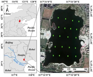
This study selected a small urban lake with an area of 0.6 km2 (600 m×1 000 m). The lake is located in an industrial park in the City of Tianjin, China, and provides flood control and ecological balance
for its surrounding areas (Figure 2). The total developed area of the industrial park is 2 km2 with
diversified land uses, including industrial, residential, and commercial areas. The ecosystem health of the lake is directly related to the management of the surrounding area.
Figure 2. Location of study area and the sampling locations (green pin labels).
Twenty sampling points were evenly distributed on the water area by the grid method. The
density of sampling points was 0.03 sites/km2. To provide simultaneous sampling with Sentinel-2,
water samples were collected by Yunzhou SE40 unmanned surface vessel (USV) at 10:00 ~ 12:00 on May 20, 2019 and June 9, 2019. The two sampling dates were selected in the early summer when aquatic plants did not grow rapidly and massively, since the aquatic plants covering the lake would impact on the retrieval accuracy. A total of 40 water samples were collected, with sampling depths of 30-50 cm. There was no cloud cover above the lake on the sampling dates. The time between sampling and satellite overpass was less than 4 hours. After being collected, water samples were quickly put into amber glass bottles to avoid sunshine, and sent to the laboratory for testing. The testing method for each parameter studied in this research is listed in Table 1. The measured water quality parameters of 40 sampling points constitute the ground truth data set.
Table 1. Testing methods.
Parameters Method
TP Acid persulfate digestion method
TN Persulfate oxidation method
COD Reactor digestion method
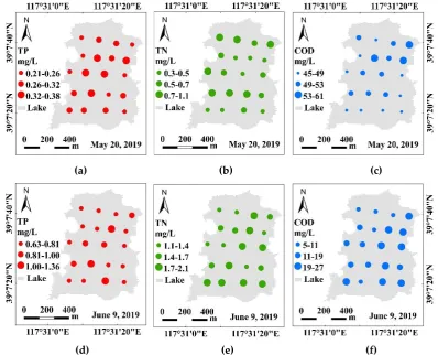
The measured water quality distribution for two sampling dates was generated by ArcGIS 10.4
(Environmental Systems Research Institute, Inc., Redlands, California, USA) .On May 20, 2019, the
mean values of TP, TN, and COD were 0.29 mg/L, 0.66 mg/L, and 50.45 mg/L, respectively. On June 9, 2019, the averages of TP and TN increased to 0.85 mg/L and 1.63 mg/L, respectively. The averages of COD decreased to 17.45 mg/L (Figure 3).
(a) (b) (c)
(d) (e) (f)
Figure 3. Distribution of measured water quality parameters. (a), (b), (c) represent TP, TN and COD,
respectively on May 20, 2019; (d), (e), (f) represent TP, TN and COD, respectively, on June 9, 2019.
2.3. Satellite data processing
Since December 3, 2015, ESA has officially provided free download services for Sentinel-2 data
to global users. Real-time updated imagery can be downloaded freely from
https://scihub.copernicus.eu. All images are acquired by multi-spectral imager (MSI). The images contain thirteen spectral bands ranging from the Visible (VNIR) and Near Infra-Red (NIR) to the Short Wave Infra-Red (SWIR). The spatial resolution of Band 2 (B2, 492.1 nm), Band 3 (B3, 559.0 nm), Band 4 (B4, 665 nm), Band 8 (B5, 833 nm) is 10 m. The spatial resolution of Band 5 (B6, 703.8 nm), Band 6 (B6, 739.1 nm), Band 7 (B7, 779.7 nm), Band 8A (B8A, 864.8 nm), Band 11 (B11, 1610.4 nm), Band 12 (B12, 2185.7 nm) is 20 m. The spatial resolution of Band 1 (B1, 442.3 nm), Band 9 (B9, 943.2 nm), Band 10 (B10, 1376.9 nm) is 60 m. Band 1, Band 9, and Band 10 are three atmospheric bands, and hence were not analyzed in this research.
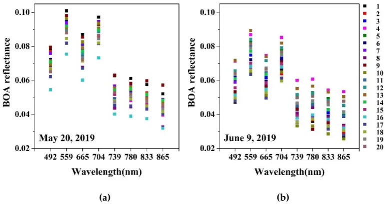
The two remote sensing images obtained in this paper were L1C products, namely atmospheric apparent reflectance products after ortho-rectification and sub-pixel geometric correction. Radiometric calibration and atmospheric correction were completed by sen2cor. Then, the L2A products were obtained, namely the bottom of atmosphere (BOA) reflectance products. Four bands with a spatial resolution of 20 m were resampled to 10 m using the Sentinel Application Platform (SNAP) v6.0, creating eight bands with a spatial resolution of 10 m (Figure 4).
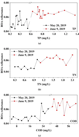
(a) (b)
Figure 4. BOA reflectance of sampling points on: (a)May 20, 2019; (b) June 9, 2019. Different colors
represent different sampling points.
Pixel values corresponding to 40 ground truth points were extracted. The entire data set for
machine learning models was composed of ‘ground truth data set’ and ‘pixel value data set’. The water area was extracted by Normalized Difference Water Index (NDWI) in ENVI 5.3 [44].
NDWI =𝑋𝐺𝑟𝑒𝑒𝑛−𝑋𝑁𝐼𝑅
𝑋𝐺𝑟𝑒𝑒𝑛+𝑋𝑁𝐼𝑅 (1)
where XGreenand XNIR are the pixel values of the green band and NIR band, respectively. For Sentinel-2 images, the green band and NIR band are B3 and B8, respectively.
2.4. Building of machine learning models
Three machine learning algorithms, namely Random Forest (RF), Support Vector Regression (SVR), and Back-Propagation Neural Networks (NN), were selected to construct regression models between water quality parameters and pixel values, respectively. The entire data set was randomly
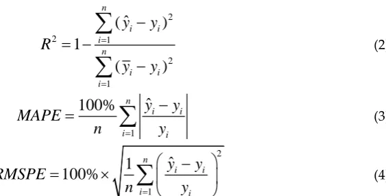
split into 70% training set and 30% test set. The coefficient of determination R-squared (R2), mean
2 2 1 2 1
ˆ
(
)
1
(
)
n i i i n i i iy
y
R
y
y
= =−
= −
−
(2)1
ˆ
100%
n i i i iy
y
MAPE
n
=y
−
=
(3)2 1
ˆ
1
100%
n i i i iy
y
RMSPE
n
=y
−
=
(4)where
y
i,y
i andy
ˆ
i stand for the measured, mean and estimated water quality parameters,respectively; and n stands for the number of sampling points. Learning curves were used to optimize
model parameters. Cross validation was used to calculate the evaluation metrics of model performance [45]. For each cross validation, the whole data set was randomly split into 70% training set and 30% test set. A model was fitted on the training set and evaluated for the test set. The final R2, MAPE, RMSPE were the average of 10 cross validations. The principles of the three machine learning algorithms are described in the following subsections.
2.4.1. Random Forest
Random Forest (RF) is an ensemble learning method [46,47]. It uses data to construct multiple models, and integrates the modeling results of all models by voting (classification problem) or taking mean (regression problem), so that the results of the entire model have high accuracy and generalization performance. In the implementation of RF, an equal number of training samples are randomly extracted from all samples, then m sub-feature sets are selected from all input features, and finally, an optimal attribute is selected from the sub-feature set for node splitting.
When solving regression problems, each decision tree is a regression tree, which is divided by the minimum mean square deviation. In other words, for splitting feature A, the corresponding arbitrary splitting point s splits the data set into two data sets (D1 and D2), so that the mean square deviation of the two data sets after splitting is minimum. The formula is as follows:
1 2
2 1
2 2
, 1 2
min min
(
)
min
(
)
( , )
( , )
i i
A s i i
y
c
y
c
c
x D A s
x D A s
c
−
+
−
(5)where c1 and c2 are the sample output mean values of D1 and D2, respectively.
y
i is themeasured value.
Then, at the two nodes after splitting, the splitting continues according to this principle. The final prediction result is the mean of all decision trees. In this research, RF was implemented by scikit-learn 0.21.3 of Python 3.7, and the main parameters were set as follows by scikit-learning curves:
Table 2. Main parameter settings of RF.
Parameters TP TN COD
n_estimators 80 36 40
max_depth 6 5 3
max_features 5 2 6
2.4.2. Support Vector Regression
SVR maps x in low-dimensional space to a high-dimensional feature space φ(x) with a non-linear
y = ⟨𝑤𝜑(𝑥)⟩ + b (6)
where x and y are the input and output. ⟨𝑤𝜑(𝑥)⟩ is the inner product of the feature space, and
the weight vector 𝑤 and bias constant b can be obtained by minimizing the risk function (7):
min (‖𝑤‖2
2 + C ∑ 𝐿𝜀
𝑁
𝑖=1 (𝑥𝑖, 𝑦𝑖, 𝑓)) (7)
In function (7):
𝐿𝜀(𝑥𝑖, 𝑦𝑖, 𝑓) = {
|𝑦𝑖− 𝑓(𝑥𝑖)| − 𝜀, |𝑦𝑖− 𝑓(𝑥𝑖)| ≥ 𝜀
0,𝑜𝑡ℎ𝑒𝑟𝑤𝑖𝑠𝑒 (8)
where 𝐿𝜀 is the loss function. C is a pre-set penalty coefficient, which is used to punish errors
greater than 𝜀. 𝜀 is the deviation between the estimated and the measured values. N is the number
of sampling points. By introducing slack variables 𝜉𝑖 and 𝜉𝑖∗, the solution of (7) can be transformed to (9):
min (‖𝑤‖2
2 + 𝐶 ∑ (𝜉𝑖+ 𝜉𝑖 ∗) 𝑁
𝑖=1 ) (9)
The constraint condition is as follows:
𝑦𝑖− [(𝑤 × 𝑥𝑖) + 𝑏] ≤ 𝜀 + 𝜉𝑖
[(𝑤 × 𝑥𝑖) + 𝑏] − 𝑦𝑖≤ 𝜀 + 𝜉𝑖∗ (10)
𝜉𝑖∗, 𝜉𝑖≥ 0
Lagrange multiplier 𝛼𝑖 and 𝛼𝑖∗ are introduced to establish Lagrange function and then solve
the dual problems of the original problems. Finally, the regression function of the optimal hyperplane is obtained:
𝑓(x) = ∑𝑁𝑖=1(𝛼𝑖− 𝛼𝑖∗)𝐾(𝑥𝑖, 𝑥) + 𝑏 (11)
where 𝐾(𝑥𝑖, 𝑥) is the kernel function:
𝐾(𝑥𝑖, 𝑥) = 𝜑⟨𝑥𝑖, 𝑥⟩ = φ(𝑥𝑖)𝑇𝜑(𝑥) (12)
The most commonly used kernel functions include: linear kernel, polynomial kernel, sigmoid kernel, radial basis function (RBF) kernel, etc. [50]. Using learning curve, RBF was selected as the
kernel function in this research:
𝐾(𝑥𝑖, 𝑥) = 𝑒−‖𝑥−𝑥𝑖‖2 𝜎
2
⁄ (13)
In this research, SVR is implemented by scikit-learn 0.21.3 of Python 3.7, and the main parameters were set as follows by learning curves:
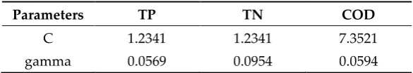
Table 3. Main parameter settings of SVR
Parameters TP TN COD
C 1.2341 1.2341 7.3521
gamma 0.0569 0.0954 0.0594
2.4.3. Neural Networks
Back-Propagation NN is a multi-layer perceptron model, which is trained by error back propagation algorithm. The model is built according to the internal relations of the data itself, and
has good non-linear approximation ability and comprehensive processing ability for cluttered information. The model structure consists of one input layer, one or more hidden layers and one
The number of nodes in the input layer (n), hidden layer (l) and output layer (m) are determined
by the sequence of input and output(X,Y). The training process of the model employs the following
steps:
1. Initialization
Initialize 𝑤𝑖𝑗 and 𝑤𝑗𝑘. 𝑤𝑖𝑗 is the connection weight between the jth neuron in the input layer and the ith neuron in the hidden layer. 𝑤𝑗𝑘 is the connection weight between the kth neuron in hidden layer and the jth neuron in the output layer. The thresholds a and b of hidden layer and output layer are preset, giving the activation function of neurons and learning efficiency 𝜂.
2. Hidden layer output calculation
The output H of the hidden layer is calculated according to the input variable X, the connection weight 𝑤𝑖𝑗 between the input layer and the hidden layer and the threshold a of the hidden layer:
𝐻𝑗= 𝑓(∑𝑛𝑖=1𝑤𝑖𝑗𝑥𝑖− 𝑎𝑗)𝑗 = 1,2, … , 𝑙 (14)
3. Output layer calculation
The predicted output O is calculated according to the output H of the hidden layer, the connection weight 𝑤𝑗𝑘 and the threshold b:
𝑂𝑘 = ∑𝑙𝑗=1𝐻𝑗𝑤𝑗𝑘− 𝑏𝑘𝑘 = 1,2, … , 𝑚 (15)
4. Error calculation
The prediction error e is calculated according to the predicted output O and the expected output Y. If the error meets the requirement, the training will be completed, otherwise step 5 will be repeated.
5. Updating weights and thresholds
Turn back to step 2 after updating the connection weight 𝑤𝑖𝑗, 𝑤𝑗𝑘 and thresholds a, b according to error e.
The common activation functions in Back-Propagation NN are ReLU function, sigmoid function
and tanh function. Among them, ReLU function is the most commonly used [51]. It is a piecewise linear function, and makes up for the gradient disappearance problem of sigmoid function and tanh
function. The function is as follows:
g(z) = {𝑧, 𝑧 > 00, 𝑧 < 0 (16)
In this research, NN is implemented in Keras 2.2.4 of Python 3.7. The number of neurons in the input layer was set to six, for there are six input bands of the remote sensing imagery. By comparing the error of training results and analyzing the calculation efficiency, the number of hidden layer was set to four. For TP and TN, the number of neurons in each hidden layer was 300. For COD, the number of neurons in each hidden layer was 200.
3. Results
3.1. Bands selection
(a)
(b)
(c)
Figure 5. The average spectral shape across the concentrations of TP (a), TN (b) and COD (c). BOA
reflectance was the average of eight bands.When plotting, different average BOA reflectance
corresponding to the same concentration were averaged.
the range of concentrations. It was suggested that the above band composition could be used to retrieve water quality parameters.
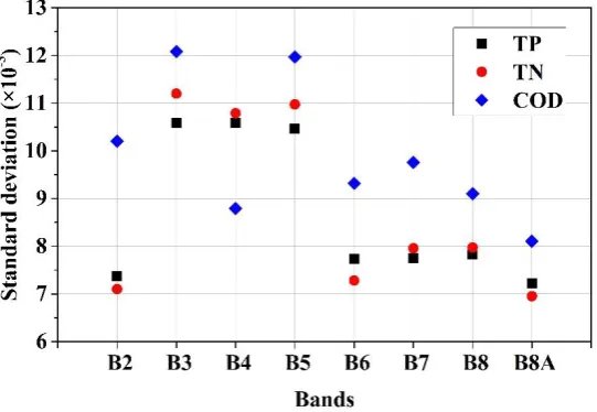
Figure 6. The standard deviation of each band across the concentrations of each water quality
parameter. The black square, red dot and blue diamond stands for TP, TN and COD, respectively.
In order to evaluate whether the above-mentioned band composition was most appropriate, this study used all possible band compositions (a total of 255 band compositions) to retrieve each water
quality parameter by multiple linear regression. R2 was selected to evaluate the model performance
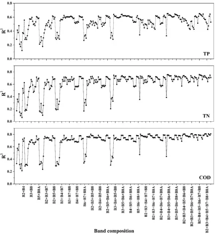
Figure 7. The R2 of each water quality parameter retrieval by different band composition.
According to Figure 7, with the increase of band number, the average R2 increased, and reached
the maximum when band number was 6. The average R2 of 7 band composition was greater than that
of 8 band composition. The most important bands were B3, B4, and B5, namely, the green and red band (B5 is the vegetation red edge with a wavelength of 705 nm). The results were consistent with
the work of Tan et al. [30]. Spectra from phytoplankton dominated water experienced low reflectance
in red (650~750 nm) wavelengths due to the absorption by Chl-a and other pigments. For the sediment dominated spectra, the reflectance values are relatively high in the green (543~578 nm) and red
(650~750 nm) wavelengths. Based on the average R2, the most appropriate band compositions of TP,
TN and COD retrieval were 'B3+B4+B5+B6+B7+B8', 'B3+B4+B5+B6+B7+B8' and 'B2+B3+B5+B6+B7+B8'.
3.2. Performance of machine learning models
Subsection 3.1. By comparing the estimated water quality parameters from models with the ground
truth, the scatter plots in Figure 8 were obtained. The average R2, MAPE, and RMSPE of 10 cross
validations was used to evaluate the performance of the models.
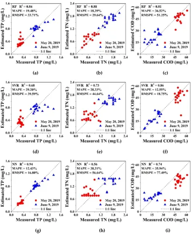
(a) (b) (c)
(d) (e) (f)
(g) (h) (i)
Figure 8. The model performance of TP, TN and COD retrieval. (a), (b), (c) represent the accuracy of
RF; (d), (e), (f) represent the accuracy of SVR; and (g), (h), (i) represent the accuracy of NN. The red
dots and blue triangles represent data sets acquired from water samples collected on May 20, 2019
and June 9,2019, respectively.
The optimal models of TP, TN and COD were quite different. For TP, the performances of NN
was good. R2 reached 0.94, and the MAPE and RMSPE were 12.43% and 16.80%, respectively. For TN,
the performances of RF was good. R2 reached 0.88, and the MAPE and RMSPE were 18.39% and
29.64%, respectively. For COD, the performances of SVR was good. R2 reached 0.86, and the MAPE
and RMSPE were 12.55% and 18.75%, respectively.
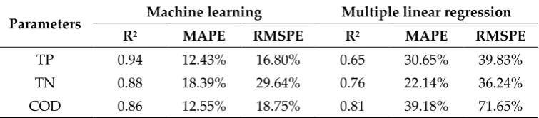
Table 4. Comparison of accuracy between machine learning and multiple linear regression.
Parameters Machine learning Multiple linear regression
R2 MAPE RMSPE R2 MAPE RMSPE
TP 0.94 12.43% 16.80% 0.65 30.65% 39.83%
TN 0.88 18.39% 29.64% 0.76 22.14% 36.24%
COD 0.86 12.55% 18.75% 0.81 39.18% 71.65%
According to Figure 8, the scatter points of each water quality parameter are obviously concentrated in two regions. Especially for TP and TN, there is almost no overlap between the two regions. This is because the water quality parameters on the two sampling dates are quite different. The magnitudes of TP and TN on June 9, 2019 were significantly higher than those on May 20, 2019, while COD on June 9, 2019 was significantly lower than that on May 20, 2019. The decrease of COD may be due to the active metabolism of microorganisms in water and the accelerated degradation of organic matter with the gradual increase of temperature.
(a)
(b)
(c)
Figure 9. Comparison of measured and estimated water quality parameters. (a), (b), (c) represent
TP, TN and COD, respectively. The black and red dots represent the estimated values by training set
and test set, respectively. The gray square represents the measured values.
3.3. Water quality mapping
(a) (b) (c)
(d) (e) (f)
Figure 10. Water quality mapping on two sampling dates. (a), (b), (c) represent TP, TN and COD,
respectively, on May 20, 2019; (d), (e), (f) represent TP, TN and COD, respectively, on June 9, 2019.
The spatial distributions of TP and TN tended to be consistent, which might be due to the fact that TP and TN were from the same pollution sources. For example, domestic sewage from residential areas was discharged into the lake. TP and TN in the south and west of the lake were higher than those in the north and east of the lake. On May 20, 2019, the high values of TP and TN were distributed in the southwest of the lake, while on June 9, 2019, the areas expanded from the southwest of the lake to the north of the lake. Accordingly, the averages of TP and TN increased from 0.29 mg/L and 0.66 mg/L on May 20, 2019 to 0.85 mg/L and 1.63 mg/L on June 9, 2019, respectively. COD in the east was higher than that in the west of the lake. On May 20, 2019, the high values of COD were distributed in most areas except the southwest of the lake. By June 9, 2019, the area of high values contracted eastward to the middle and east of the lake. Meanwhile, the averages of COD decreased from 50.45 mg/L on May 20, 2019 to 17.45 mg/L on June 9, 2019.
According to the mapping of TP and TN, domestic sewage containing N and P might be continuously discharged into the lake. It was observed from the remote sensing images that there
was a piece of farm land with an area about 1.25 km2 as well as a subdivision of a residential area
It could be observed that water quality parameters were not evenly distributed, although the waterbody was fairly small (surface area was 0.6 km2 and less than 1 km2). The study of water quality retrieval based on high resolution satellite image is therefore crucial for many water management issues, e.g. identifying illegal discharges to urban waterbody, spills on the shore etc.
4. Discussion
4.1 Assessment of water quality conditions
Comparing the estimated water quality parameters to the environmental quality standards for
surface water (National Standard of the People’s Republic of China, GB3838-2002), the Figure 11 was obtained. The environmental quality standards for surface water classified each water quality parameter into five levels, i.e., Class I~V from good water quality to poor.
(a) (b) (c) Figure 11. Comparison of estimated water quality parameters and the environmental quality
standards for surface water (National Standard of the People’s Republic of China, GB3838-2002). (a),
(b), (c) represent TP, TN and COD, respectively. The red dashed lines represent different
classifications of water quality (noted with Roman numerals).
According to Figure 11, TP on both May 20, 2019 and June 9, 2019 was worse than Class V. Serious phosphorus pollution existed in the entire lake surface. TN of the lake surface on both May 20, 2019 and June 9, 2019 covered from Class II to V. The average TN on both May 20, 2019 and June 9, 2019 was subject to Class IV. On May 20, 2019, 1.05%, 40.37%, 21.33% and 37.25% of the lake surface was subject to Class II, Class III, Class IV and Class V. On June 9, 2019, the water quality deteriorated. Class III, Class IV and Class V area expanded to 28.63%, 25.65% and 74.35%. Class II area almost disappeared. COD of the lake surface on both May 20, 2019 and June 9, 2019 covered from Class II to V. In part of the lake surface, COD was worse than Class V. The average COD on both May 20, 2019 and June 9, 2019 was subject to Class V. On May 20, 2019, 41.21% of the lake surface was worse than Class V. 4.29%, 9.10%, 19.09% and 26.30% of the lake surface was subject to Class I~II, Class III, Class IV and Class V, respectively. On June 9, 2019, area with COD worse than Class V decreased to 34.49%. Area of Class V and Class II decreased to 22.43% and 3.8%,
respectively. Area of Class III and Class IV increased to 11.44% and 27.84%, respectively.
4.2 Comparison of retrieval accuracy
Figure 12. R2 comparison of existing publications and this research. The min, lower quartile,
median, upper quartile, max and mean of the R2 of existing retrieval for TP, TN and COD were
displayed by Box-plot. Theasterisk represents the retrieval R2 in this research.
Since the average R2 of TP in the existing publications [21,22,24–27,29] was 0.653, the performance of TP retrieval was improved by about 44% over the average of the past research works. For TN, the average R2 in the existing publications [21,23–27] was 0.613, and the performance of TN retrieval in this research was improved by 43% over the average of the past research works. For COD, the average R2 in the past research works [17–20] was 0.722, and the performance of retrieval COD in this research was slightly higher than the upper quartile of the past research works. Based on the above analysis, the performance of water quality retrieval in this research has improved by using a combination of machine learning strategies. As the key nutrient for eutrophication, TP has the highest performance. The machine learning strategy proposed in this study may help in water quality management for urban waterbodies.
5. Conclusions
This research developed a machine learning based monitoring method for non-optically active water quality parameters of small urban waterbodies based on Sentinel-2 imagery. The main conclusions are as follows:
1. This is the first attempt to retrieve water quality parameters for small waterbodies with surface area less than 1 km2.
2. Compared with TM/ETM+, MODIS and other data, Sentinel-2 with high spatiotemporal
resolution makes it possible to retrieve the water quality characteristics for small urban waterbodies.
3. The most important Sentinel-2 bands of TP, TN and COD retrieval were B3, B4, and B5. The
optimal retrieval accuracy of TP, TN and COD was acquired from the band compositions of 'B3+B4+B5+B6+B7+B8', 'B3+B4+B5+B6+B7+B8' and 'B2+B3+B5+B6+B7+B8', respectively.
4. The performances of water quality retrieval for these non-optically active parameters were
significantly improved by the optimized machine learning models, especially TP and TN.
5. According to the water quality mapping by remote sensing and the interview of the
residents in the neighborhood, the pollutants, especially the illegal discharges of industrial effluent, were traced back to the source.
Funding: The National Key Research and Development Program of China (2016YFC0400709), Ministry of Science and Technology of the People’s Republic of China and Science.
Technology Commission of Tianjin Binhai New Area (BHXQKJXM-PT-ZJSHJ-2017001).
Acknowledgments: This research was supported by The National Key Research and Development Program of China (2016YFC0400709), Ministry of Science and Technology of the People’s Republic of China and Science and
Technology Commission of Tianjin Binhai New Area (BHXQKJXM-PT-ZJSHJ-2017001).
Conflicts of Interest: The authors declare no conflict of interest.
References
1. Shao, M.; Tang, X.; Zhang, Y.; Li, W. City clusters in China: Air and surface water pollution. Front. Ecol.
Environ. 2006.
2. Hoekstra, A.Y.; Buurman, J.; Van Ginkel, K.C.H. Urban water security: A review. Environ. Res. Lett.
2018.
3. Brönmark, C.; Hansson, L.A. Environmental issues in lakes and ponds: Current state and perspectives.
Environ. Conserv. 2002, 29, 290–307.
4. Shuchman, R.A.; Sayers, M.; Fahnenstiel, G.L.; Leshkevich, G. A model for determining
satellite-derived primary productivity estimates for Lake Michigan. J. Great Lakes Res. 2013.
5. Ritchie, J.C.; Zimba, P. V.; Everitt, J.H. Remote sensing techniques to assess water quality. Photogramm.
Eng. Remote Sensing 2003.
6. O’Reilly, J.E.; Maritorena, S.; Mitchell, B.G.; Siegel, D.A.; Carder, K.L.; Garver, S.A.; Kahru, M.;
McClain, C. Ocean color chlorophyll algorithms for SeaWiFS. J. Geophys. Res. Ocean. 1998.
7. Olmanson, L.G.; Brezonik, P.L.; Bauer, M.E. Airborne hyperspectral remote sensing to assess spatial
distribution of water quality characteristics in large rivers: The Mississippi River and its tributaries in
Minnesota. Remote Sens. Environ. 2013.
8. Ritchie, J.C.; Schiebe, F.R.; McHenry, J.R. Remote sensing of suspended sediments in surface waters.
Photogramm. Remote SENS. 1976.
9. Holyer, R.J. Toward universal multispectral suspended sediment algorithms. Remote Sens. Environ.
1978.
10. Duan, H.; Ma, R.; Hu, C. Evaluation of remote sensing algorithms for cyanobacterial pigment retrievals
during spring bloom formation in several lakes of East China. Remote Sens. Environ. 2012.
11. Shuchman, R.A.; Leshkevich, G.; Sayers, M.J.; Johengen, T.H.; Brooks, C.N.; Pozdnyakov, D. An
algorithm to retrieve chlorophyll, dissolved organic carbon, and suspended minerals from Great Lakes
satellite data. J. Great Lakes Res. 2013.
12. Andrzej Urbanski, J.; Wochna, A.; Bubak, I.; Grzybowski, W.; Lukawska-Matuszewska, K.; Łącka, M.;
Śliwińska, S.; Wojtasiewicz, B.; Zajączkowski, M. Application of Landsat 8 imagery to regional-scale
assessment of lake water quality. Int. J. Appl. Earth Obs. Geoinf. 2016.
13. Shi, K.; Zhang, Y.; Zhu, G.; Liu, X.; Zhou, Y.; Xu, H.; Qin, B.; Liu, G.; Li, Y. Long-term remote
monitoring of total suspended matter concentration in Lake Taihu using 250 m MODIS-Aqua data.
Remote Sens. Environ. 2015.
14. Brezonik, P.L.; Olmanson, L.G.; Finlay, J.C.; Bauer, M.E. Factors affecting the measurement of CDOM
by remote sensing of optically complex inland waters. Remote Sens. Environ. 2015.
15. Lei, X.; Pan, J.; Devlin, A.T. Characteristics of absorption spectra of chromophoric dissolved organic
16. Hou, X.; Feng, L.; Duan, H.; Chen, X.; Sun, D.; Shi, K. Fifteen-year monitoring of the turbidity
dynamics in large lakes and reservoirs in the middle and lower basin of the Yangtze River, China.
Remote Sens. Environ. 2017.
17. Wang, Y.; Xia, H.; Fu, J.; Sheng, G. Water quality change in reservoirs of Shenzhen, China: Detection
using LANDSAT/TM data. Sci. Total Environ. 2004.
18. Sharaf El Din, E.; Zhang, Y.; Suliman, A. Mapping concentrations of surface water quality parameters
using a novel remote sensing and artificial intelligence framework. Int. J. Remote Sens. 2017.
19. Deng, C.; Zhang, L.; Cen, Y. Retrieval of chemical oxygen demand through modified capsule network
based on hyperspectral data. Appl. Sci. 2019.
20. El-Rawy, M.; Fathi, H.; Abdalla, F. Integration of remote sensing data and in situ measurements to
monitor the water quality of the Ismailia Canal, Nile Delta, Egypt. Environ. Geochem. Health 2019, 5.
21. He, W.; Chen, S.; Liu, X.; Chen, J. Water quality monitoring in a slightly-polluted inland water body
through remote sensing - Case study of the Guanting Reservoir in Beijing, China. Front. Environ. Sci.
Eng. China 2008, 2, 163–171.
22. Chang, N. Bin; Xuan, Z.; Yang, Y.J. Exploring spatiotemporal patterns of phosphorus concentrations in
a coastal bay with MODIS images and machine learning models. Remote Sens. Environ. 2013.
23. Lim, J.; Choi, M. Assessment of water quality based on Landsat 8 operational land imager associated
with human activities in Korea. Environ. Monit. Assess. 2015, 187, 1–17.
24. Gholizadeh, M.H.; Melesse, A.M. Study on Spatiotemporal Variability of Water Quality Parameters in
Florida Bay Using Remote Sensing. J. Remote Sens. GIS 2017, 06.
25. Li, Y.; Zhang, Y.; Shi, K.; Zhu, G.; Zhou, Y.; Zhang, Y.; Guo, Y. Monitoring spatiotemporal variations in
nutrients in a large drinking water reservoir and their relationships with hydrological and
meteorological conditions based on Landsat 8 imagery. Sci. Total Environ. 2017, 599–600, 1705–1717.
26. Mathew, M.M.; Srinivasa Rao, N.; Mandla, V.R. Development of regression equation to study the Total
Nitrogen, Total Phosphorus and Suspended Sediment using remote sensing data in Gujarat and
Maharashtra coast of India. J. Coast. Conserv. 2017.
27. Wang, D.; Cui, Q.; Gong, F.; Wang, L.; He, X.; Bai, Y. Satellite retrieval of surface water nutrients in the
coastal regions of the East China Sea. Remote Sens. 2018.
28. Xiong, J.; Lin, C.; Ma, R.; Cao, Z. Remote sensing estimation of lake total phosphorus concentration
based on MODIS: A case study of Lake Hongze. Remote Sens. 2019, 11, 1–19.
29. Xiong, Y.; Ran, Y.; Zhao, S.; Zhao, H.; Tian, Q. Remotely assessing and monitoring coastal and inland
water quality in China: Progress, challenges and outlook. Crit. Rev. Environ. Sci. Technol. 2019, 0, 1–37.
30. Tan, J.; Cherkauer, K.A.; Chaubey, I. Developing a comprehensive spectral-biogeochemical database of
midwestern rivers for water quality retrieval using remote sensing data: A case study of the Wabash
River and its tributary, Indiana. Remote Sens. 2016.
31. Chen, J.; Quan, W. Using Landsat/TM imagery to estimate nitrogen and phosphorus concentration in
Taihu Lake, China. IEEE J. Sel. Top. Appl. Earth Obs. Remote Sens. 2012.
32. Moses, W.J.; Gitelson, A.A.; Perk, R.L.; Gurlin, D.; Rundquist, D.C.; Leavitt, B.C.; Barrow, T.M.;
Brakhage, P. Estimation of chlorophyll-a concentration in turbid productive waters using airborne
hyperspectral data. Water Res. 2012.
33. Moses, W.J.; Gitelson, A.A.; Berdnikov, S.; Povazhnyy, V. Satellite estimation of chlorophyll-a
concentration using the red and NIR bands of MERISThe azov sea case study. IEEE Geosci. Remote Sens.
34. Gitelson, A.A.; Gao, B.C.; Li, R.R.; Berdnikov, S.; Saprygin, V. Estimation of chlorophyll-a
concentration in productive turbid waters using a Hyperspectral Imager for the Coastal Ocean - The
Azov Sea case study. Environ. Res. Lett. 2011.
35. Duan, H.; Ma, R.; Loiselle, S.A.; Shen, Q.; Yin, H.; Zhang, Y. Optical characterization of black water
blooms in eutrophic waters. Sci. Total Environ. 2014.
36. Halme, E.; Pellikka, P.; Mõttus, M. Utility of hyperspectral compared to multispectral remote sensing
data in estimating forest biomass and structure variables in Finnish boreal forest. Int. J. Appl. Earth Obs.
Geoinf. 2019.
37. Kishino, M.; Tanaka, A.; Ishizaka, J. Retrieval of Chlorophyll a, suspended solids, and colored
dissolved organic matter in Tokyo Bay using ASTER data. Remote Sens. Environ. 2005.
38. Liu, R.; Chen, Y.; Sun, C.; Zhang, P.; Wang, J.; Yu, W.; Shen, Z. Uncertainty analysis of total
phosphorus spatial-temporal variations in the Yangtze River Estuary using different interpolation
methods. Mar. Pollut. Bull. 2014.
39. Moses, W.J.; Gitelson, A.A.; Berdnikov, S.; Povazhnyy, V. Estimation of chlorophyll-a concentration in
case II waters using MODIS and MERIS data - Successes and challenges. Environ. Res. Lett. 2009.
40. Brando, V.E.; Dekker, A.G. Satellite hyperspectral remote sensing for estimating estuarine and coastal
water quality. IEEE Trans. Geosci. Remote Sens. 2003.
41. Li, J.; Hu, C.; Shen, Q.; Barnes, B.B.; Murch, B.; Feng, L.; Zhang, M.; Zhang, B. Recovering low quality
MODIS-Terra data over highly turbid waters through noise reduction and regional vicarious
calibration adjustment: A case study in Taihu Lake. Remote Sens. Environ. 2017.
42. Wang, S.; Li, J.; Zhang, B.; Spyrakos, E.; Tyler, A.N.; Shen, Q.; Zhang, F.; Kuster, T.; Lehmann, M.K.;
Wu, Y.; et al. Trophic state assessment of global inland waters using a MODIS-derived Forel-Ule index.
Remote Sens. Environ. 2018.
43. Le, C.; Li, Y.; Zha, Y.; Sun, D.; Huang, C.; Zhang, H. Remote estimation of chlorophyll a in optically
complex waters based on optical classification. Remote Sens. Environ. 2011.
44. McFeeters, S.K. The use of the Normalized Difference Water Index (NDWI) in the delineation of open
water features. Int. J. Remote Sens. 1996.
45. Rapinel, S.; Mony, C.; Lecoq, L.; Clément, B.; Thomas, A.; Hubert-Moy, L. Evaluation of Sentinel-2
time-series for mapping floodplain grassland plant communities. Remote Sens. Environ. 2019, 223, 115–
129.
46. Mutanga, O.; Adam, E.; Cho, M.A. High density biomass estimation for wetland vegetation using
worldview-2 imagery and random forest regression algorithm. Int. J. Appl. Earth Obs. Geoinf. 2012.
47. Wang, Y.; Du, Y.; Wang, J.; Li, T. Calibration of a low-cost PM2.5 monitor using a random forest
model. Environ. Int. 2019, 133, 105161.
48. Vapnik, V.N. The Nature of Statistical Learning Theory. Springer-Verlag; 1995; ISBN 0-471-03003-1.
49. Mountrakis, G.; Im, J.; Ogole, C. Support vector machines in remote sensing: A review. ISPRS J.
Photogramm. Remote Sens. 2011.
50. Chen, J.; de Hoogh, K.; Gulliver, J.; Hoffmann, B.; Hertel, O.; Ketzel, M.; Bauwelinck, M.; van
Donkelaar, A.; Hvidtfeldt, U.A.; Katsouyanni, K.; et al. A comparison of linear regression,
regularization, and machine learning algorithms to develop Europe-wide spatial models of fine
particles and nitrogen dioxide. Environ. Int. 2019, 130.
51. Kurt, A.; Gulbagci, B.; Karaca, F.; Alagha, O. An online air pollution forecasting system using neural